Chapter 8 Predicting site location with simple additive raster sensitivity analysis using R
Matthew Harris
8.0.1 Simple Arbitrary Additive Weight Sensitivity Model
This code demonstrates the process for building a simple arbitrary weight archaeological sensitivity model, selecting a model threshold, and model validation. This type of model is by no means the ‘best’ model for archaeological predictive modeling, but it is very common, a useful approach to sensitivity stratification, as well as a good example of working with raster data and model validation.
The primary use for this approach is:
- Stratify areas of a landscape based on the additive arbitrary sensitivity weights of one or more variables.
Some advantages include:
- Conceptually simple; easy to explain
- based on expert opinion
- Computationally simple
- Not based on sample of known sites
- Sidesteps some bias in site sampling
Some drawbacks include:
- Central Limit Theorem challenges statistical basis
- Difficult to optimize
- Not based on sample of known sites
- No method for assessing variable importance
- Does not include the variation evident in known site locations
Primary R techniques used in this script:
- reading/writing raster files
- using the raster package in R (e.g. reclassify, mask, etc…)
- Interactive maps with mapview package
- Creating your own function
- plotting with ggplot2
8.0.2 Study Area
This study area is a relatively large study area (897336 raster cells at 10.63425 meter resolution, for 101,477,305 square meters) including 120 pre-contact archaeological sites from somewhere in the United States. The coordinates of the data have been altered to protect the location of the sites. For the purpose of mapping, the coordinates of the data have been relocated to map over Fargo, North Dakota. In an ideal world, more site location data would be free…
8.0.3 Code
The code below follows the sequence of defining functions and packages, loading raster data, establishing weights, classifying rasters based on weights, summing all weighted rasters, validating with known site locations, plotting results.
8.0.4 Define functions
I typically put all my functions at the beginning of my code once I have them in working order. Here I define a function that takes the predicted sensitivity and presence/absence of known sites and returns a series of performance metrics to demonstrate how well the model classifies known sites. This function utilizes the ROCR package to define performance metrics across all thresholds.
# predict == predicted value from model raster
# response == site present (1) or site absent (0) at each predicted cell location
balance_threshold <- function(predict, response) {
  perf <- ROCR::performance(ROCR::prediction(predict, response), "sens", "spec")
  auc <- ROCR::performance(ROCR::prediction(predict, response), "auc")
  auc <- round(auc@y.values[[1]],3)
  df <- data.frame(Weight = perf@alpha.values[[1]],
                   Spec = perf@x.values[[1]],
                   Sens = perf@y.values[[1]],
                   Back_pcnt = 1 - perf@x.values[[1]],
                   Xover = abs((perf@y.values[[1]] + (1-perf@x.values[[1]]))-1))
  df$kg <- 1-((1-df$Spec)/df$Sens)
  df$reach <- 1-((1-df$Sens)/df$Spec)
  df$reach <- ifelse(df$reach == 1, 0, df$reach) # removing reach == 1
  df <- data.frame(apply(df,2,function(x) round(x,3)))
  sens_spec <- df[which.max(df$Sens + df$Spec), "Weight"]
  xover <- df[which.min(df$Xover), "Weight"]
  kg <- df[which.max(df$kg), "Weight"]
  reach <- df[which.max(df[which(df$reach < 1),"reach"]), "Weight"] # max where it is not == 1
  list(df = df, sens_spec = sens_spec, xover = xover,
       auc = auc, kg = kg, reach = reach)
}
8.0.5 Load packages
I also typically put all of the necessary packages at the top of my code and typically note why I used that package in a comment. Otherwise, I will forget for some of the less common packages. Using R typically requires using a series of packages for any analysis. This is a strength of R, but requires one to learn how various packages work and to find the package for the task at hand. Don’t be worried about using a bunch of packages, but try to keep the updated!
library("raster")       # for raster manipulation
library("rgdal")        # for raster processing
library("dplyr")        # for data processing
library("mapview")      # for interactive map plots
library("ggplot2")      # for plotting results
library("ROCR")         # for model validation functions
library("RColorBrewer") # for raster color scale
library("knitr")        # for printing nicer tables
library("viridis")      # for color scale in ggplot
8.0.6 Load raster files
The raster package is the workhorse of dealing with raster data in R. It is a large an complex package, but has good documentation and is pretty easy to learn. The files used here were saved as .tif files from ArcGIS. A critical part of making this work is to make sure that you set your environments in ArcGIS or QGIS to align the grid cells for each raster, use the same projection, and consistently mask the raster so they have the same number of rows and columns. This can all be done in R, but to simplify this script, I did it in ArcGIS and exported to tif files.
The raster stack is a raster data structure that combines rasters of the same dimension into a single file for ease of use. This includes running one operation that works on each raster in the stack; as we will see.
Variables:
- slope.tif is the percent slope of the landscape derived from a 1/3rd arc-second DEM
- ed_h2.tif is the euclidean distance to National Hydrology Dataset (NHD) stream features
- ed_h4.tif is the euclidean distance to National Wetland Dataset (NWD) wetland polygons
- sites.tif is the location of
120known archaeological site as rasterized polygons
data_loc <- "clip_raster/"
slope <- raster(paste0(data_loc, "slope.tif"))
ed_h2 <- raster(paste0(data_loc, "ed_h2.tif"))
ed_h4 <- raster(paste0(data_loc, "ed_h4.tif"))
sites <- raster(paste0(data_loc, "sites.tif"))
raster_vars <- stack(slope, ed_h2, ed_h4, sites)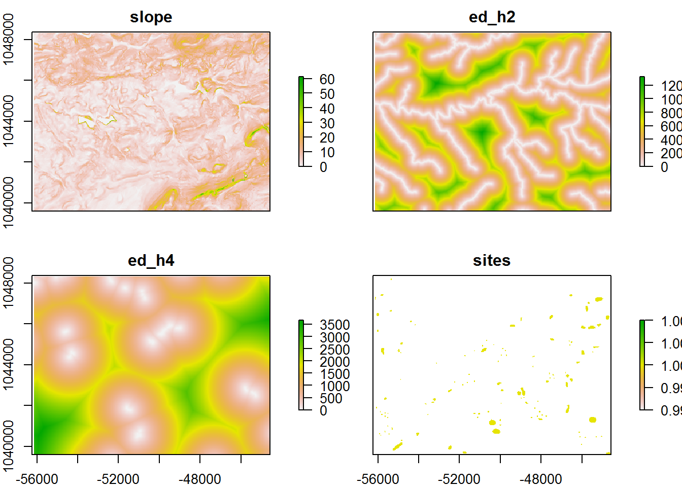
8.0.7 Construct weights
The core component of this model is the establishing of arbitrary weights assigned to classes of each raster variable. These weights can be based on educated guesses, empirical evidence, or to test a theory. Likewise, the manner in which the raster is classified into regions to weight is equally arbitrary or empirically based. What is not happening here is the use of known data to find the optimum set of weights and data splits to best separate site locations from non-sites. That is a model that discriminates based on known sites and weights from a metric such as information value or through statistical means of classification such as logistic regression, random forests, or any number of models.
Here, the weights and splits are based on regional literature for how micro-social camps type sites are possibly distributed relative to these variables. Known site locations obviously influence this understanding, but they are not directly calculated to create the weights. The structure of these tables needs to be three columns that depict the values of form, to, and value. These are the raster values to classify from and to and the weight to assign to that class.
### Slope weighting Models###
slp_from <- c(0, 3, 5, 8, 15)
slp_to   <- c(3, 5, 8, 15, 99999)
slp_wght <- c(50, 30, 15, 5, 0)
slp_rcls<- cbind(slp_from, slp_to, slp_wght)

### Dist to h20 weighting Models###
h20_from <- c(0, 100, 200, 400, 800)
h20_to   <- c(100, 200, 400, 800, 9999)
h20_wght <- c(60, 25, 10, 4, 1)
h20_rcls <- cbind(h20_from, h20_to, h20_wght)

### Dist to wetland weighting Models###
wtl_from <- c(0, 100, 200, 400, 800)
wtl_to   <- c(100,200, 400, 800, 9999)
wtl_wght <- c(35, 25, 20, 15, 5)
wtl_rcls <- cbind(wtl_from, wtl_to, wtl_wght)

print(slp_rcls)
## slp_from slp_to slp_wght
## [1,] 0 3 50
## [2,] 3 5 30
## [3,] 5 8 15
## [4,] 8 15 5
## [5,] 15 99999 0print(h20_rcls)## h20_from h20_to h20_wght
## [1,] 0 100 60
## [2,] 100 200 25
## [3,] 200 400 10
## [4,] 400 800 4
## [5,] 800 9999 1# an example of a more fully formatted table
knitr::kable(wtl_rcls, digits = 0,
col.names = c("From", "To", "Weight"),
caption = "Sensitivity Weights for Distance (m) to Wetlands (NWD)")| From | To | Weight |
|---|---|---|
| 0 | 100 | 35 |
| 100 | 200 | 25 |
| 200 | 400 | 20 |
| 400 | 800 | 15 |
| 800 | 9999 | 5 |
8.0.8 Reclassify rasters
The code to reclassify the rasters is very straight forward. For each of the three variable, we indicate that particular raster from the stack using the indexing of a list and the weight table. The reclassify function in the raster package does the work for us.
raster_vars[["slope"]] <- reclassify(raster_vars[["slope"]], slp_rcls)
raster_vars[["ed_h2"]] <- reclassify(raster_vars[["ed_h2"]], h20_rcls)
raster_vars[["ed_h4"]] <- reclassify(raster_vars[["ed_h4"]], wtl_rcls)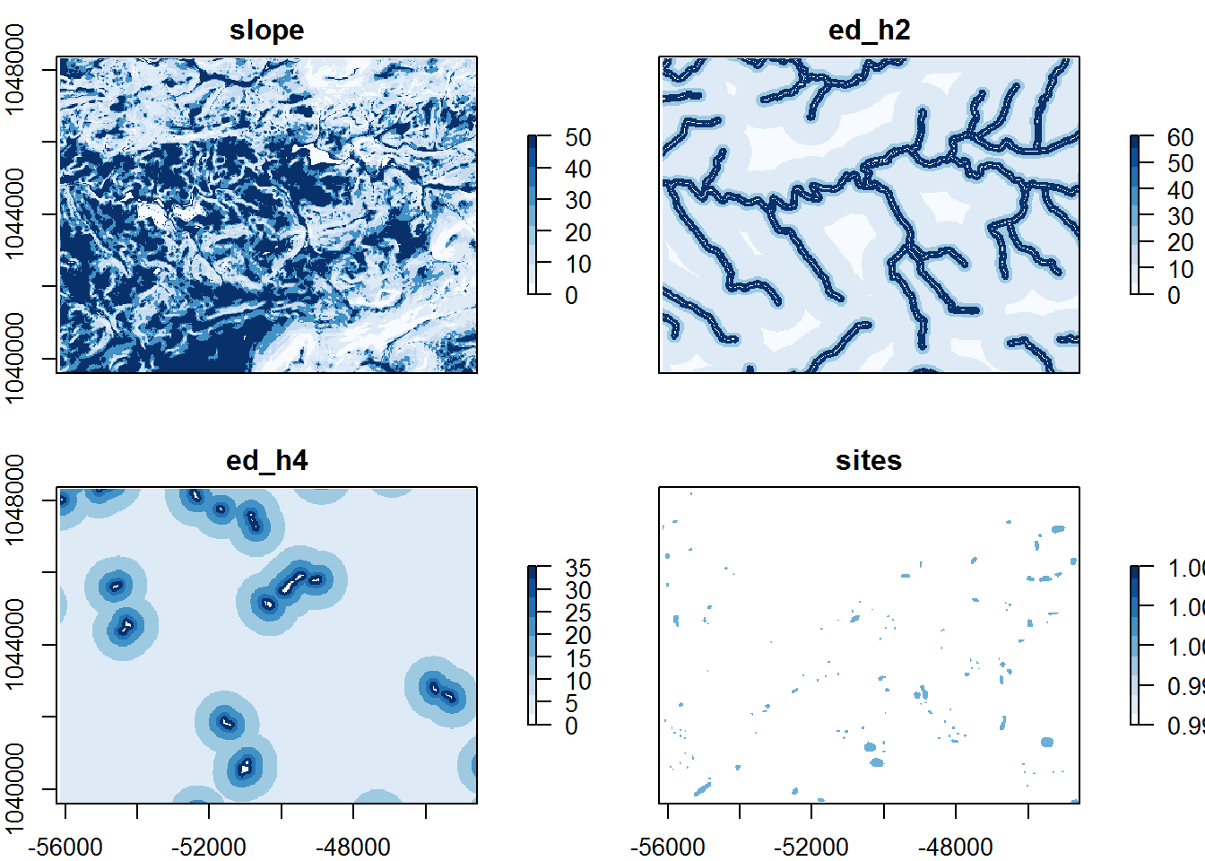
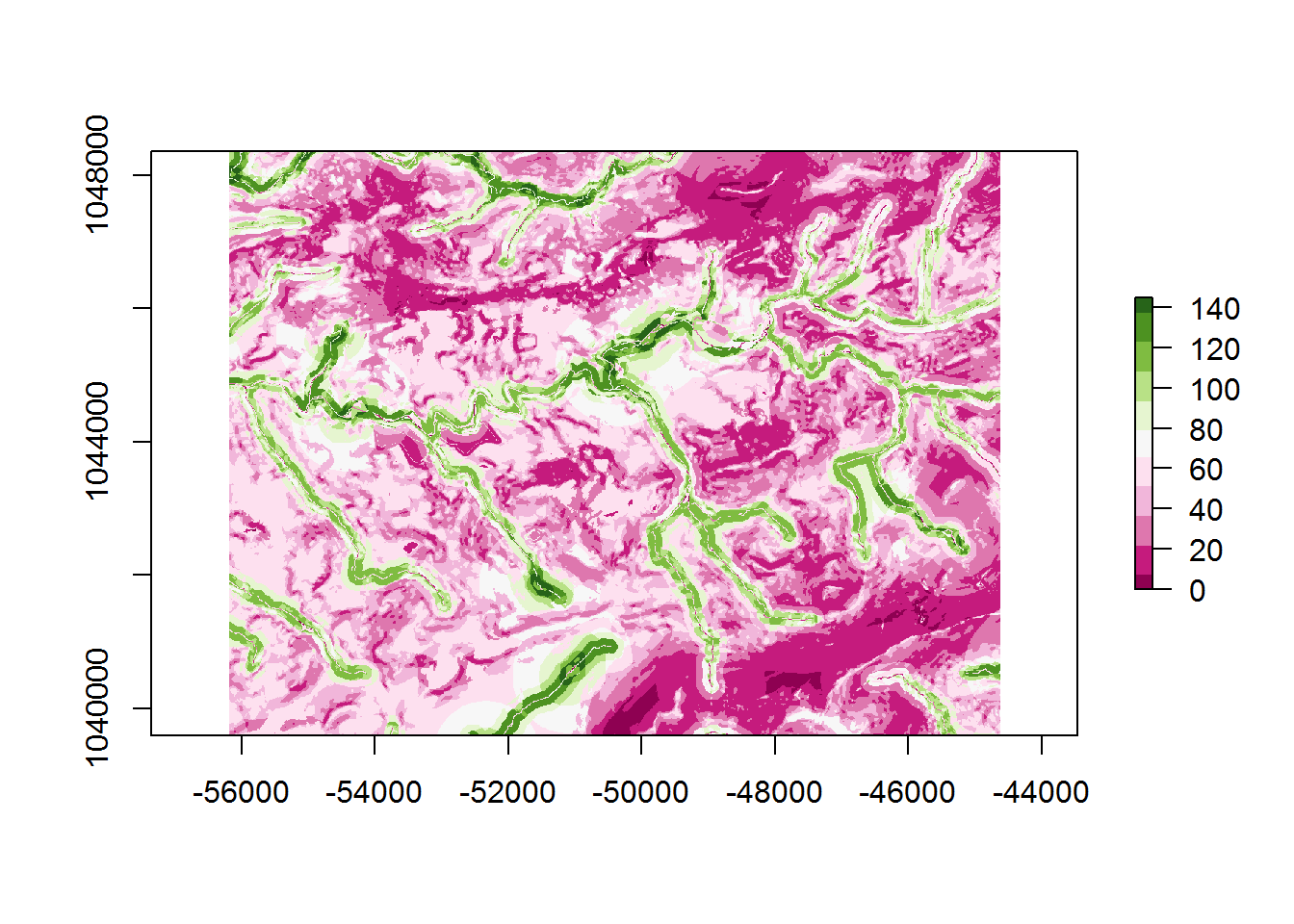
8.0.9 Summing rasters
Given that the weighted rasters are within the raster stack, the sum() function will add together all of the layers that we indicate; in this case [1:3]. These are the weighted slope, ed_h2, and ed_h4 rasters.
model_sum <- sum(raster_vars[[1:3]])base plot of model_sum
ggplot of model_sum
coords <- coordinates(model_sum)
x <- data.frame(x = coords[,"x"], y = coords[,"y"], value = as.vector(model_sum))
ggplot(x, aes(x = x, y = y, fill = value)) +
  geom_raster(hjust = 0, vjust = 0) +
  theme_minimal() +
  viridis::scale_fill_viridis() +
  labs(title = "Summed Sensitivity Weights",
       caption = "Projection: Albers Conic Equal Area")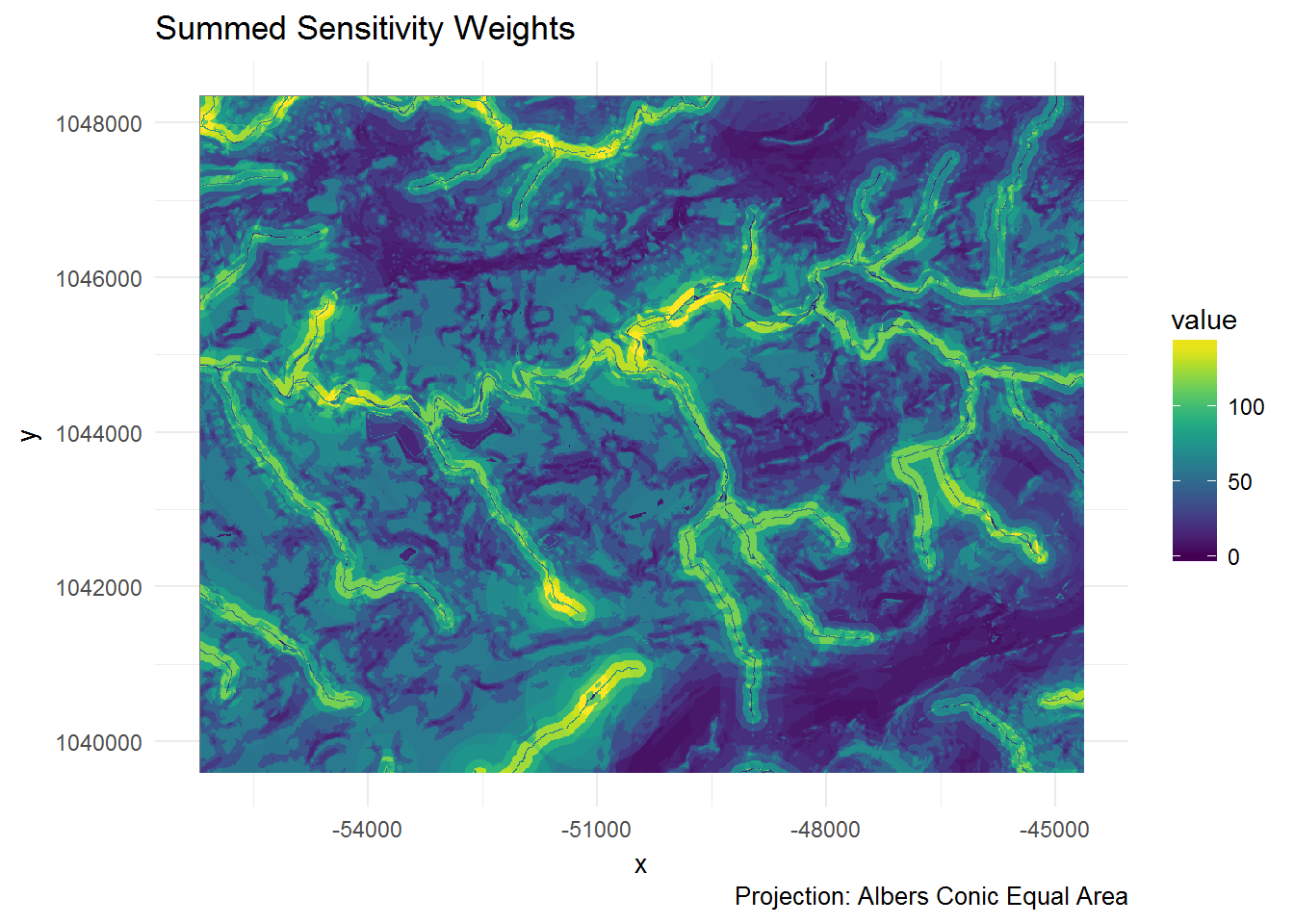
8.0.10 Clip sites
In order to validate the weighting scheme and assess model performance, it is necessary to find out the summed weight value at known site locations. With this information, one can see if the summed weights are able to discriminate the parts of the landscape that are known to contain sites vs. the summed weights of the study area overall. Ideally, a model will give high summed weights to where sites are known and lower weights on average to where there are no sites; e.g. the background. However, since the purpose of this model is to identify areas of site potential/sensitivity, we need it to have some areas of high summed weights, but no known sites. The trick of any model type is to balance the size of this false-positive area (until survey proves otherwise) against the false-positive areas where we misclassify sites as absent. Further along we will use performance metrics to try to find the weight threshold that achieves this balance.
The mask() function of the raster package is used to clip the summed weight raster model_sum by the known site locations.
sites_sum <- mask(model_sum, raster_vars[["sites"]])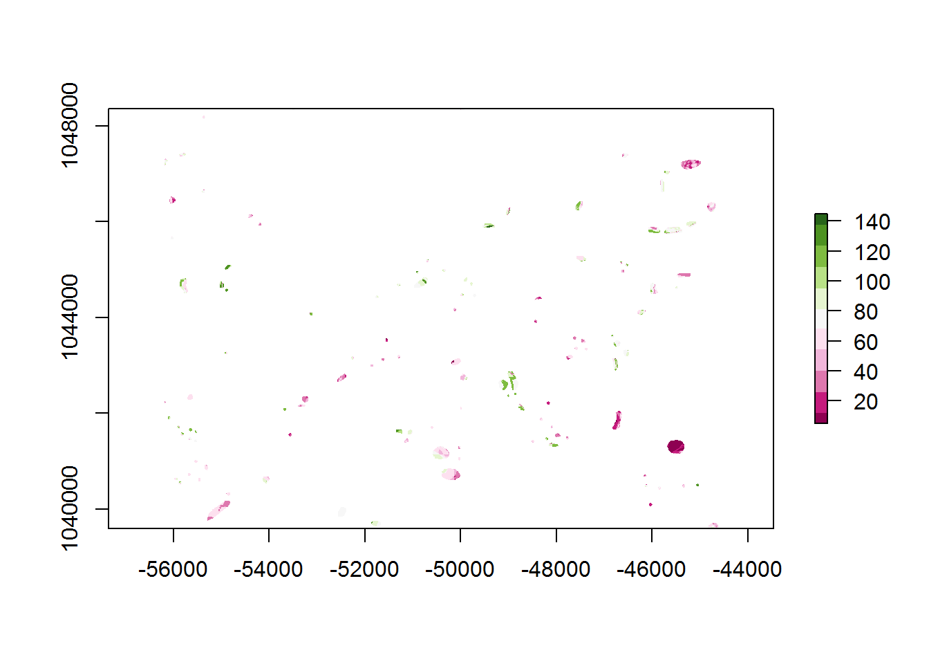
8.0.10.1 Mapview
Spatial data can be easily rendered in a ‘slippy-map’ format with the mapview package. This allows for overlays, base maps, legends, zooming, and panning with a very easy to use function.
m <-  mapview(model_sum,
              col.regions = viridisLite::viridis,
              alpha = 0.75, maxpixels =  897336) +
      mapview(sites_sum,
              col.regions = viridisLite::magma,
              maxpixels =  897336)
m
8.0.11 Model Validation
“All models a wrong, but some are useful” ~ G. Box
Box goes on to explain this in detail later by adding that a model’s usefulness is dependent on its purpose. Further, its purpose should not be figured out after the model is built. This understanding of purpose -> mechanism -> model -> validation is important in framing the model building process.
Model validation is a hugely important topic and deserve a thorough treatment on its own. However, we will cover a basic validation here by comparing the model’s ability to distinguish the location of known sites form the environmental background, as well as quantifying the balance of model errors vs. success. The former is important in understanding the model’s bias and the latter important in balancing the models variance. See this post for a great introduction.
8.0.11.1 Model discrimination
If your study area has known sites, they can be used to test how well the model isolates the location of known sites and potentially the locations of yet-to-be-known sites. If known sites in your study area were used to derive the model weights, then this process should utilize a set of test sites that are held out from the model construction. Other techniques such as k-folds cross-validation, bootstrapping, and generalization error estimations are common approaches in approximating unbiased model performance.
In this demo the model performance is based on the choice of model variables and the weights assigned to them. Based on the assumptions that we chose variables that are able to distinguish where settlement has occurred and that we assigned higher weights to areas of the landscape that are more likely to contain sites, our expectation is that when the score are summed, known sites will map on to higher weighted areas than the environmental background. To test this, we can extract the weights from the model_sum and sites_sum raster layers and plot the density of weights for each.
# build a data.frame of weights and assign labels for sites and background
sum_dat <- data.frame(wght = c(model_sum@data@values, sites_sum@data@values),
                      model = c(rep("background", length(model_sum)),
                                rep("site", length(sites_sum)))) %>%
  mutate(class = ifelse(model == "site", 1, 0)) %>%
  na.omit()

# plot the wieghts as a density to compare
ggplot(sum_dat, aes(x = wght, group = model, fill = model)) +
  geom_density(alpha = 0.55, adjust = 2) +
  scale_x_continuous(limits = c(0,200), expand = c(0, 0)) +
  scale_y_continuous(expand = c(0, 0)) +
  labs(x="Summed Weight", y="Density",
       title="Density of Summed Weights by Class") +
theme_bw() 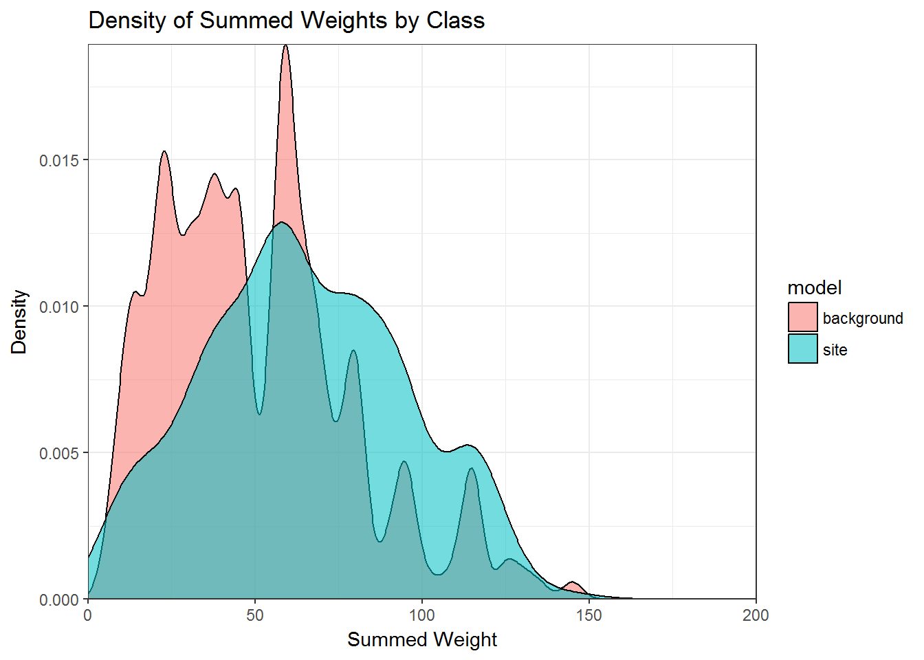
Or as a boxplot…
# plot the wieghts as a boxplots to compare
ggplot(sum_dat, aes(x = model, y = wght, group = model, fill = model)) +
  geom_boxplot() +
  labs(x="Classification", y="Summed Weight",
       title="Summed Weights by Class") +
theme_bw() 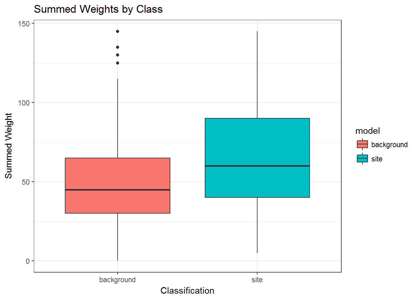
8.0.11.2 Performance and thresholds
In the section above, we performed simple model validation to visually assess the bias in of the model, or to put it another way, how well the model approximates the general sensitivity of settlement locations given variables, weights, and test site locations. Clearly there could be better weights, different variables, other test site samples, or no signal/mechanism to be found. The model’s success or failure to validate is not dependent on what could be, but what is based on the above vis a vis the model’s purpose. If the model’s bias is too great to achieve the model’s purpose given your assumptions, then you will need to reevaluate. If the model appears to be approaching your desired target, then now is a good time to assess its performance.
In a classification model, performance depends on choosing thresholds. This is one of the most important yet glossed-over topics across many modeling applications. The summed weights of our model give a continuous distribution of values, however in a classification setting is it desirable to split these weights into present vs. absent, or high, medium, and low classes. An example of how threshold and performance are related and why it is so important is as follows. If a client asked me to make a model of sensitivity, I can guarantee them a perfect model that never fails. I do this by setting my present/absent threshold at model_sum == 0. I can guarantee that this model will identify the location of every unknown site only because it classifies the entire study are as site-likely. Sure, the client had to survey every square-meter of the study area, but every site will be found (assuming 100% identifiability). Of course, everyone knows this is not how the real world works and in this scenario, there is no reason to even make a model!
Alternatively, if the client has a very slim budget, I can pick a threshold model_sum == max(model_sum) that classifies the entire study area as site-unlikely and I can guarantee that no site will be found. Of course, this is terrible from an archaeologist’s point of view, but it illustrates that the “best” threshold is somewhere in the middle. We can find that middle ground through various means, though the general approach is to balance the two extremes to optimize one or numerous metrics. Below we will evaluate for the metrics of Sensitivity, Specificity, Area Under the Curve (AUC), and the classic Kvamme Gain. Wikipedia has a good overview of Sensitvity, Specificity, and realted metrics.
Below we use the performance() and prediction() functions in the ROCR package to derive the model’s Sensitivity (true positive rate) and Specificity (true negative rate) at each a threshold for each summed weight. So in this model, there are 54 unique combinations of weights, so it calculates 55 values for sensitivity and specificity. We also calculates a series of metrics that can be used to obtain a threshold value on which to classify site-likely vs. site-unlikely. They are: Kvamme Gain, Xover, Sens-Spec, and reach.
# model_pred <- prediction(sum_dat$wght, sum_dat$class) %>%
#   performance(., "sens", "spec")

model_pref <- balance_threshold(sum_dat$wght, sum_dat$class)
Kvamme Gain (KG) is a classic threshold metric in APM defined as 1 - (% background / % sites) which translates to 1 - ((1 - Specificity) / Sensitivity). The Reach metric is essentially the inverse of the KG, 1 - ((1 - Sensitvity) / Specificity), Sens-Spec is threshold that maximizes for both sensitivity and specificity, and Xover is the balance of sensitivity and specificity; this is the threshold illustrated by Kvamme (1998, pg 391, figure 8.11(B)). Each of these threshold give us a different justification for our model and which we chose should depend on any number of criteria including the model itself, use of the model, policy implications, funding, research, etc… for this demo, we will be using Xover as the balance of the true positive and true negative error rates.
To visualize these thresholds and the trade-off they represent, we can plot how sensitivity and specificity change across each potential threshold value (weight) and overlay the four thresholds introduced above. To plot this, the output from the balance_threshold() function needs to be formatted into a long format using tidy::gather().
xover_dat <-  tidyr::gather(model_pref$df, metric, value, -Weight, -kg, -Back_pcnt, -Xover, -reach)
threshold_dat <- data.frame(threshold = c("kg", "reach", "X-over", "Sens-Spec"),
                            weight =  c(model_pref$kg, model_pref$reach, model_pref$xover, model_pref$sens_spec))
ggplot() +
  geom_line(data = xover_dat, aes(x = Weight, y = value, group = metric, color = metric), size=1) +
  geom_linerange(data = threshold_dat, aes(x = weight, ymin = 0, ymax = 1, linetype = threshold)) +
  scale_x_continuous(breaks=seq(0,200,5), labels = seq(0,200,5)) +
  scale_y_continuous(breaks=seq(0,1,0.1), labels = seq(0,1,0.1)) +
  labs(title = "Sensitivity and Specificity at Optimized Metrics") +
  theme_bw() +
  theme(
    axis.text.x = element_text(angle = 90, hjust = 1)
  )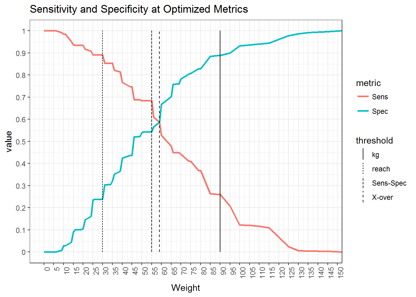
From this plot, we can see that:
- The KG threshold optimizes to maximize the amount of background relative to correct site predictions
- The reach threshold optimizes to maximize the percent correct sites over background
- The Sens-Spec threshold maximizes both sensitivity and specificity together, and
- The Xover threshold finds the point at which the sensitivity equals specificity
Xover and Sens-Spec will typically be pretty close to each other and KG and reach will typically be biased towards background and sites respectively. In this demo we will assume that the maximization of sensitivity and specificity represented Sens-Spec achieves our goals and proceed with using the summed weight value of 55 to classify the model into site-likely and site-unlikely. This is achieved using the raster::reclassify() function as used earlier to weight the rasters.
class_rcls <- matrix(c(-Inf, model_pref$sens_spec, 0,
                       model_pref$sens_spec, Inf, 1), ncol=3, byrow=TRUE)
model_class <- reclassify(model_sum, class_rcls, right = FALSE)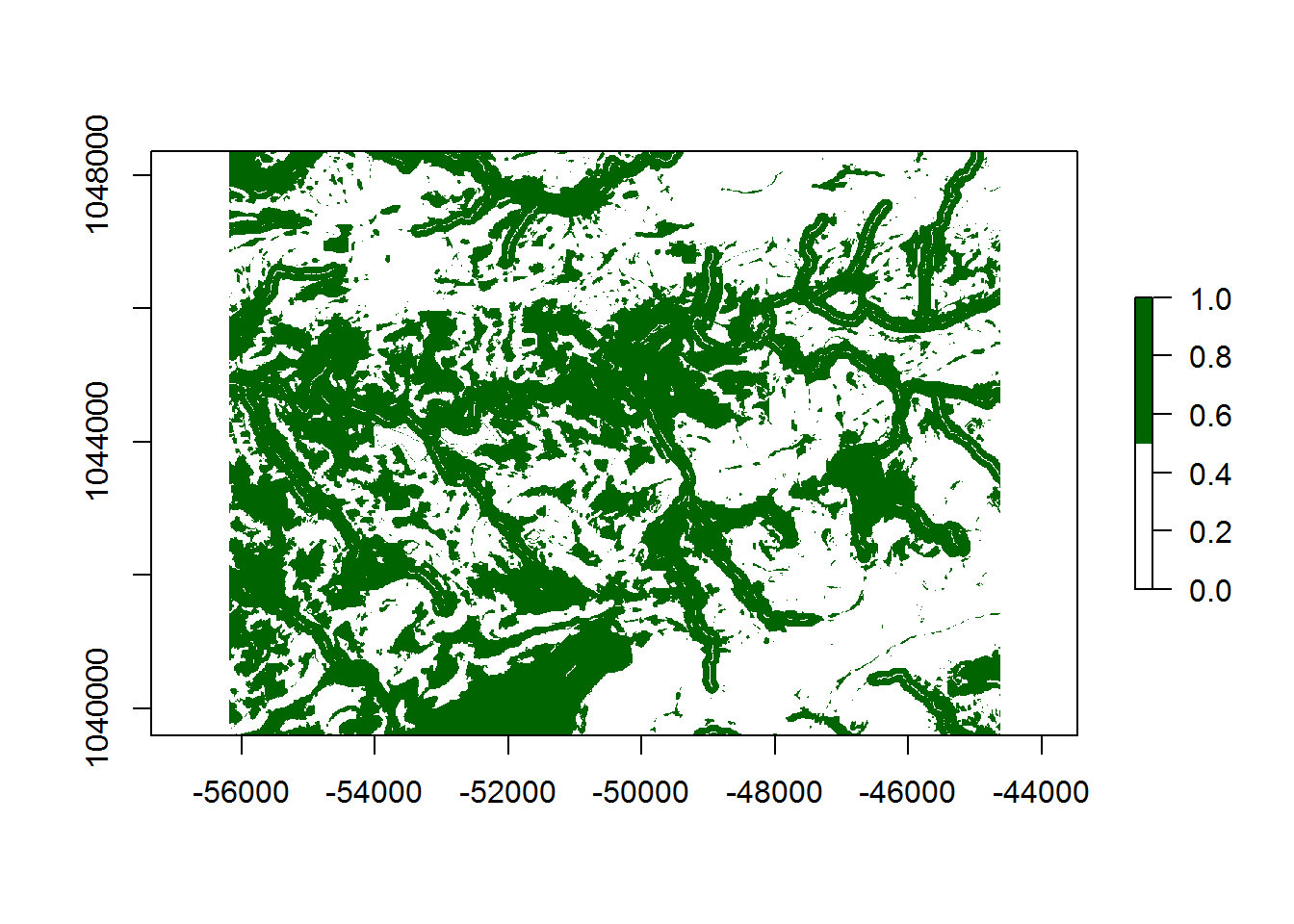
8.0.12 Results
Based on the model and the chosen threshold, we can quantify the results in terms of the percent of site-present cells (not specifically % of total sites in this case) defined by sensitivity versus the percent of the model classified as site-likely defined as 1 - specificity (calculated as Back-pcnt in the table below). With this specific model, we are able to correctly classify 68.4 percent of the known site-present raster cells within 45.6 percent of the study area, for a KG of 0.334
model_pref[["df"]] %>%
  dplyr::filter(Weight == model_pref$sens_spec)
## Weight Spec Sens Back_pcnt Xover kg reach
## 1 55 0.544 0.684 0.456 0.139 0.334 0.4198.0.12.1 Final Model
The final classified raster and sites are rendered with mapview(). *unfortunately this is not rendering in the knit R markdown version
m <- mapview(model_class,
             col.regions = viridisLite::viridis,
             alpha = 0.75,
             maxpixels =  897336) +
     mapview(sites_sum,
             col.regions = viridisLite::magma,
             maxpixels =  897336)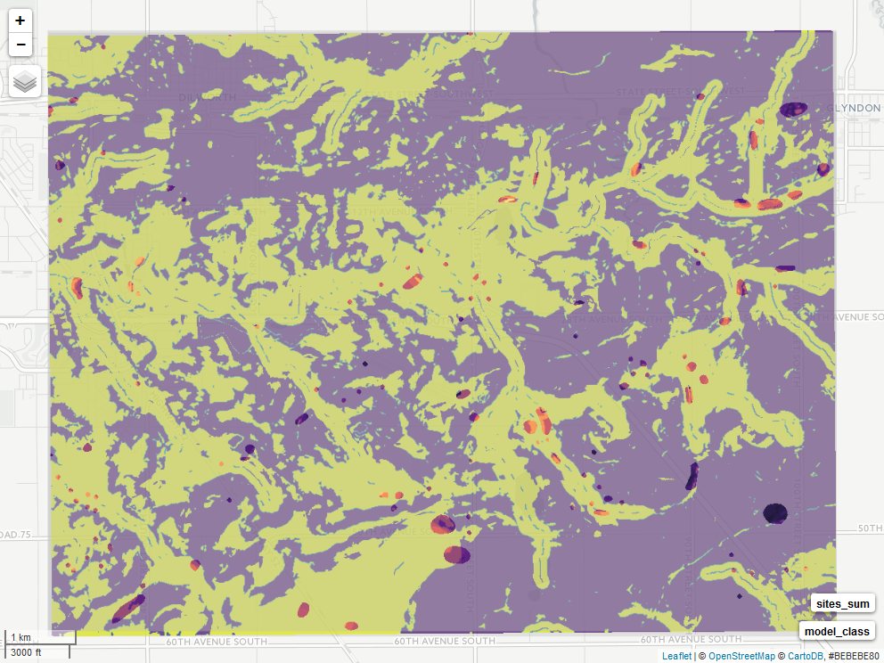
8.0.12.2 sessionInfo()
environment parameters
sessionInfo()## R version 3.3.3 (2017-03-06)
## Platform: x86_64-w64-mingw32/x64 (64-bit)
## Running under: Windows 7 x64 (build 7601) Service Pack 1
##
## locale:
## [1] LC_COLLATE=English_Australia.1252 LC_CTYPE=English_Australia.1252
## [3] LC_MONETARY=English_Australia.1252 LC_NUMERIC=C
## [5] LC_TIME=English_Australia.1252
##
## attached base packages:
## [1] methods stats graphics grDevices utils datasets base
##
## other attached packages:
## [1] viridis_0.4.0 viridisLite_0.2.0 knitr_1.15.17
## [4] RColorBrewer_1.1-2 ROCR_1.0-7 gplots_3.0.1
## [7] ggplot2_2.2.1 mapview_1.2.0 leaflet_1.1.0
## [10] dplyr_0.5.0 rgdal_1.2-5 raster_2.5-8
## [13] sp_1.2-4
##
## loaded via a namespace (and not attached):
## [1] gtools_3.5.0 lattice_0.20-34 colorspace_1.3-2
## [4] htmltools_0.3.5 stats4_3.3.3 base64enc_0.1-3
## [7] yaml_2.1.14 R.oo_1.21.0 DBI_0.6
## [10] R.utils_2.5.0 foreach_1.4.3 plyr_1.8.4
## [13] stringr_1.2.0 munsell_0.4.3 gtable_0.2.0
## [16] R.methodsS3_1.7.1 htmlwidgets_0.8 caTools_1.17.1
## [19] codetools_0.2-15 evaluate_0.10 labeling_0.3
## [22] latticeExtra_0.6-28 httpuv_1.3.3 crosstalk_1.0.0
## [25] gdalUtils_2.0.1.7 highr_0.6 Rcpp_0.12.10
## [28] KernSmooth_2.23-15 xtable_1.8-2 backports_1.0.5
## [31] scales_0.4.1 satellite_0.2.0 gdata_2.17.0
## [34] jsonlite_1.3 webshot_0.4.0 mime_0.5
## [37] gridExtra_2.2.1 png_0.1-7 digest_0.6.12
## [40] stringi_1.1.3 bookdown_0.3.16 shiny_1.0.0
## [43] grid_3.3.3 rprojroot_1.2 bitops_1.0-6
## [46] tools_3.3.3 magrittr_1.5 lazyeval_0.2.0
## [49] tibble_1.2 tidyr_0.6.1 assertthat_0.1
## [52] rmarkdown_1.4 iterators_1.0.8 R6_2.2.0