Chapter 9 Landscape-based Hypothesis Testing in R
Kyle Bocinsky
9.1 Introduction
Many region-scale analyses in archaeology begin with a simple question: How do site locations relate to landscape attributes, such as elevation, soil type, or distance to water or other resources. Such a question is the foundation of basic geospatial exploratory data analysis, and answering it for a set of landscape attributes is the first step towards doing more interesting things, from interpreting settlement patterns in the past (Kowalewski 2008), to the construction of sophisticated predictive models of site location (Graves McEwan 2012; Kohler and Parker 1986; Maschner and Stein 1995), to guiding settlement decision frameworks in agent-based simulations (e.g., Axtell et al. 2002; Griffin and Stanish 2007; Kohler and Varien 2012). In this tutorial, we will learn how to use R to load, view, and explore site location data, and perform a very basic statistical settlement pattern analysis relating site location to elevation.
Of course, archaeological site locations are often sensitive information, and it wouldn’t be prudent to provide them in tutorial like this. So instead of using cultural site locations, we’ll use a point dataset for which we can make a reasonable hypothesis concerning landscape attributes: cell tower locations from the US Federal Communications Commission. The cell tower data are somewhat difficult to work with, so I’ve distilled a snapshot of the database (accessed on February 14, 2017), and posted it online for easy download. We’ll go through the process of downloading them later in this tutorial. The hypothesis we’ll be testing is that cell towers are positioned in unusually high places on the landscape. This is similar to hypotheses we might make about archaeological site locations, perhaps having to do with defensibility (e.g., Bocinsky 2014; Martindale and Supernant 2009; Sakaguchi, Morin, and Dickie 2010) or intervisibility and signaling (e.g., Johnson 2003; Van Dyke et al. 2016).
This tutorial is an R Markdown HTML document, meaning that all of the code to perform the calculations presented here was run when this web page was built—the paper was compiled. “Executable papers” such as this one are fantastic for presenting reproducible research in such a way that data, analysis, and interpretation are each given equal importance. Feel free to use this analysis as a template for your own work. All data and code for performing this analysis are available on Github at https://github.com/bocinsky/r_tutorials.
9.2 Learning goals
In this short tutorial, you will learn how to:
- Download files from the internet in R
- Read ESRI shapefiles and other spatial objects into R using the
sfandrasterpackages - Promote tabular data to spatial objects
- Crop spatial objects by overlaying them atop one another
- Generate interactive web-maps using the
leafletpackage - Download federated datasets (including elevation data) using the
FedDatapackage - Extract data from a raster for specific points
- Calculate and graph Monte Carlo sub-sampled kernel density estimates for random locations
- Calculate Monte Carlo sub-sampled Mann-Whitney U test statistics (a non-parametric equivalent to the Student’s t-test)
We will also gloss over several other fun topics in R data analysis, so download the source to learn more!
9.3 Loading necessary packages
Almost all R scripts require that you load packages that enable the functions you use in your script. We load our requisite packages here using the install_cran() function from the devtools library. install_cran() is nice because it will checck whether we have the most recent version of the packages, and only install the ones that are necessary. We also use the walk() function from the purrr package to quickly traverse a vector, but that’s a topic for another tutorial.
knitr::opts_chunk$set(echo = TRUE)

packages <- c("magrittr", # For piping
              "foreach", "purrr", "tibble", "dplyr", "tidyr", "broom", # For tidy data analysis
              "ggplot2","plotly", # For fancy graphs
              "sf", "sp", "raster", # For spatial analysis
              "leaflet", "htmltools", # For fancy maps
              "FedData")

# install.packages("devtools")
# devtools::install_cran(packages, repos = "https://cran.rstudio.com/") # For downloading federated geospatial data
purrr::walk(packages,
            library,
            character.only = TRUE) # Load all packages with no output

# Create an output folder in our current working directory
dir.create("OUTPUT",
           showWarnings = FALSE,
           recursive = FALSE)
9.4 Defining the study area
All landscape-scale analyses start with the definition of a study area. Since the cell tower dataset with which we’ll be working covers the whole USA, we could really set our study area to be anywhere in the US. Here, we will download an 1:500,500 scale ESRI shapefile of counties in the United States available from the US Census, and pick a county to serve as our study area. I’m going to pick Whitman county, Washington, because that’s where I live; feel free to choose your own county!
Files may be downloaded in R using many different functions, but perhaps the most straightforward is the download.file() function, which requires that you specify a url to the file you wish to download, and a destfile where the downloaded file should end up. As the counties shapefile is in a zip archive, we will also use the unzip() function, which requires you define an extraction directory (exdir).
# Download the 1:500000 scale counties shapefile from the US Census
if(!file.exists("OUTPUT/cb_2015_us_county_500k.zip"))
  download.file("http://www2.census.gov/geo/tiger/GENZ2015/shp/cb_2015_us_county_500k.zip",
                destfile = "OUTPUT/cb_2015_us_county_500k.zip")

# Unzip the file
unzip("OUTPUT/cb_2015_us_county_500k.zip",
      exdir = "OUTPUT/counties")
Navigate to the exdir you specified and check to make sure the shapefile is there.
Now it’s time to load the shapefile into R. We’ll be using the st_read() function from the sf library, which reads a shapefile (and many other file formats) and stores it in memory as a “simple feature” object of the sf library. To read a shapefile, the st_read() function requires only the path to the shapefile with the “.shp” file extension. Other spatial file formats have different requirements for st_read(), so read the documentation (help(st_read)) for more information.
# Load the shapefile
census_counties <- sf::st_read("OUTPUT/counties/cb_2015_us_county_500k.shp")
## Reading layer `cb_2015_us_county_500k' from data source `E:\My Documents\My Papers\conferences\SAA2017\How-To-Do-Archaeological-Science-Using-R\08_Bocinsky\OUTPUT\counties\cb_2015_us_county_500k.shp' using driver `ESRI Shapefile'
## converted into: POLYGON
## Simple feature collection with 3233 features and 9 fields
## geometry type: MULTIPOLYGON
## dimension: XY
## bbox: xmin: -179.1489 ymin: -14.5487 xmax: 179.7785 ymax: 71.36516
## epsg (SRID): 4269
## proj4string: +proj=longlat +datum=NAD83 +no_defs# Inspect the spatial object
head(census_counties)## Simple feature collection with 6 features and 9 fields
## geometry type: MULTIPOLYGON
## dimension: XY
## bbox: xmin: -88.47323 ymin: 31.18113 xmax: -85.04931 ymax: 33.00682
## epsg (SRID): 4269
## proj4string: +proj=longlat +datum=NAD83 +no_defs
## STATEFP COUNTYFP COUNTYNS AFFGEOID GEOID NAME LSAD ALAND
## 1 01 005 00161528 0500000US01005 01005 Barbour 06 2291820706
## 2 01 023 00161537 0500000US01023 01023 Choctaw 06 2365954971
## 3 01 035 00161543 0500000US01035 01035 Conecuh 06 2201896058
## 4 01 051 00161551 0500000US01051 01051 Elmore 06 1601876535
## 5 01 065 00161558 0500000US01065 01065 Hale 06 1667804583
## 6 01 109 00161581 0500000US01109 01109 Pike 06 1740741211
## AWATER geometry
## 1 50864677 MULTIPOLYGON(((-85.748032 3...
## 2 19059247 MULTIPOLYGON(((-88.473227 3...
## 3 6643480 MULTIPOLYGON(((-87.427204 3...
## 4 99850740 MULTIPOLYGON(((-86.413335 3...
## 5 32525874 MULTIPOLYGON(((-87.870464 3...
## 6 2336975 MULTIPOLYGON(((-86.199408 3...When we inspect the census_counties object, we see that it is a simple feature collection with 3233 features. Simple feature collection objects are simply data frames with an extra column for spatial objects, and metadata including projection information.
Now it’s time to extract just the county we want to define our study area. Because a Simple feature collection object extends the data.frame class, we can perform selection just as we would with a data.frame. We do that here using the filter() function from the dplyr package:
# Select Whitman county
my_county <- dplyr::filter(census_counties, NAME == "Whitman")

# Inspect the spatial object
my_county
## Simple feature collection with 1 feature and 9 fields
## geometry type: MULTIPOLYGON
## dimension: XY
## bbox: xmin: -179.1489 ymin: -14.5487 xmax: 179.7785 ymax: 71.36516
## epsg (SRID): 4269
## proj4string: +proj=longlat +datum=NAD83 +no_defs
## STATEFP COUNTYFP COUNTYNS AFFGEOID GEOID NAME LSAD ALAND
## 1 53 075 01533501 0500000US53075 53075 Whitman 06 5591999422
## AWATER geometry
## 1 47939386 MULTIPOLYGON(((-118.249122 ...As you can see, the spatial object now has only one feature, and it is Whitman county! We’ll map it in a minute, but first let’s do two more things to make our lives easier down the road. We’ll be mapping using the leaflet package, which makes pretty, interactive web maps. For leaflet, we need the spatial data to be in geographic coordinates (longitude/latitude) using the WGS84 ellipsoid. Here, we’ll transform our county to that projection system using the st_transform() function.
This code chunk also uses something new: the pipe operator %>% from the magrittr package. The pipe operator enables you to “pipe” a value forward into an expression or function call—whatever is on the left hand side of the pipe becomes the first argument to the function on the right hand side. So, for example, to find the mean of the numeric vector c(1,2,3,5) by typing mean(c(1,2,3,5)), we could instead use the pipe: c(1,2,3,5) %>% mean(). Try running both versions; you should get 2.75 for each. The pipe isn’t much use for such a simple example, but becomes really helpful for code readability when chaining together many different functions. The compound assignment operator %<>% pipes an object forward into a function or call expression and then updates the left hand side object with the resulting value, and is equivalent to x <- x %>% fun()
# Transform to geographic coordinates
my_county %<>%
  sf::st_transform("+proj=longlat +datum=WGS84")
9.5 Reading “site” locations from a table and cropping to a study area
Alright, now that we’ve got our study area defined, we can load our “site” data (the cell towers). We can use the read_csv() function from the readr library to read the cell tower locations from a local file, which we download using download.file(). We’ll read them and then print them.
# Download cell tower location data
if(!file.exists("OUTPUT/cell_towers.csv"))
  download.file("https://raw.githubusercontent.com/bocinsky/r_tutorials/master/data/cell_towers.csv",
                destfile = "OUTPUT/cell_towers.csv")

# Load the data
cell_towers <- readr::read_csv("OUTPUT/cell_towers.csv")

cell_towers
## # A tibble: 101,388 × 5
## `Unique System Identifier` `Entity Name`
## <int> <chr>
## 1 96974 Crown Castle GT Company LLC
## 2 96978 SBC TOWER HOLDINGS LLC
## 3 96979 CHAMPAIGN TOWER HOLDINGS LLC
## 4 96981 CCATT LLC
## 5 96989 Crown Atlantic Company LLC
## 6 96999 SBC TOWER HOLDINGS LLC
## 7 97007 American Towers, LLC
## 8 97011 UNITED STATES CELLULAR CORPORATION
## 9 97014 Crown Castle South LLC
## 10 97022 Crown Castle GT Company LLC
## # ... with 101,378 more rows, and 3 more variables: `Height of
## # Structure` <dbl>, Latitude <dbl>, Longitude <dbl>As you can see, the cell tower data includes basic identification information as well as geographic coordinates in longitude and latitude. We can use the coordinate data to promote the data frame to a spatial object using the st_as_sf() function. Finally, we can write a simple function to select only the cell towers in our study area using the filter() function again, along with the st_within() function from the sf package.
# Promote to a simple feature collection
cell_towers %<>%
  sf::st_as_sf(coords = c("Longitude","Latitude"),
               crs = "+proj=longlat +datum=WGS84")

# Select cell towers in our study area
cell_towers %<>%
  dplyr::filter({
    sf::st_within(., my_county, sparse = F) %>% # This function returns a matrix
                  as.vector() # coerce to a vector
    })

cell_towers
## Simple feature collection with 41 features and 3 fields
## geometry type: POINT
## dimension: XY
## bbox: xmin: -176.6418 ymin: 13.27747 xmax: -64.68769 ymax: 71.31036
## epsg (SRID): 4326
## proj4string: +proj=longlat +datum=WGS84 +no_defs
## # A tibble: 41 × 4
## `Unique System Identifier` `Entity Name`
## <int> <chr>
## 1 597094 Qwest Corporation
## 2 597409 NORTHWEST LEASE ONE, L.L.C.
## 3 597902 SINCLAIR LEWISTON LICENSEE, LLC
## 4 598225 Inland Cellular LLC
## 5 598624 AVISTA CORPORATION
## 6 598630 AVISTA CORPORATION
## 7 599225 WASHINGTON STATE UNIVERSITY
## 8 609045 UNION PACIFIC RAILROAD
## 9 612883 PALOUSE COUNTRY INC.
## 10 2606107 Washington State University
## # ... with 31 more rows, and 2 more variables: `Height of
## # Structure` <dbl>, geometry <simple_feature>Now we see that there are 41 cell towers in our study area.
9.6 Visualizing site locations
There are many different ways to visualize spatial data in R, but perhaps the most useful is using the leaflet package, which allows you to make interactive HTML maps that will impress your friends, are intuitive to a 4-year-old, and will thoroughly confuse your advisor. I’m not going to go through all of the syntax here, but in general leaflet allows you to layer spatial objects over open-source map tiles to create pretty, interactive maps. Here, we’ll initialize a map, add several external base layer tiles, and then overlay our county extent and cell tower objects. leaflet is provided by the good folks at RStudio, and is well documented here. Zoom in on the satellite view, and you can see the cell towers!
# Create a quick plot of the locations
leaflet(width = "100%") %>% # This line initializes the leaflet map, and sets the width of the map at 100% of the window
  addProviderTiles("OpenTopoMap", group = "Topo") %>% # This line adds the topographic map from Garmin
  addProviderTiles("OpenStreetMap.BlackAndWhite", group = "OpenStreetMap") %>% # This line adds the OpenStreetMap tiles
  addProviderTiles("Esri.WorldImagery", group = "Satellite") %>% # This line adds orthoimagery from ESRI
  addProviderTiles("Stamen.TonerLines", # This line and the next adds roads and labels to the orthoimagery layer
                   group = "Satellite") %>%
  addProviderTiles("Stamen.TonerLabels",
                   group = "Satellite") %>%
  addPolygons(data = my_county, # This line adds the Whitman county polygon
              label = "My County",
              fill = FALSE,
              color = "red") %>%
  addMarkers(data = cell_towers,
             popup = ~htmlEscape(`Entity Name`)) %>% # This line adds cell tower locations
  addLayersControl( # This line adds a controller for the background layers
    baseGroups = c("Topo", "OpenStreetMap", "Satellite"),
    options = layersControlOptions(collapsed = FALSE),
    position = "topleft")
It’s obvious from this map that the cell towers aren’t merely situated to be in high places—they also tend to cluster along roads and in densely populated areas.
9.7 Downloading landscape data with FedData
FedData is an R package that is designed to take much of the pain out of downloading and preparing data from federated geospatial databases. For an area of interest (AOI) that you specify, each function in FedData will download the requisite raw data, crop the data to your AOI, and mosaic the data, including merging any tabular data. Currently, FedData has functions to download and prepare these datasets:
- The National Elevation Dataset (NED) digital elevation models (1 and 1/3 arc-second; USGS)
- The National Hydrography Dataset (NHD) (USGS)
- The Soil Survey Geographic (SSURGO) database from the National Cooperative Soil Survey (NCSS), which is led by the Natural Resources Conservation Service (NRCS) under the USDA,
- The Global Historical Climatology Network (GHCN) daily weather data, coordinated by the National Oceanic and Atmospheric Administration (NOAA),
- The Daymet gridded estimates of daily weather parameters for North America, version 3, available from the Oak Ridge National Laboratory’s Distributed Active Archive Center (DAAC), and
- The International Tree Ring Data Bank (ITRDB), coordinated by NOAA.
In this analysis, we’ll be downloading the 1 arc-second elevation data from the NED under our study area. The FedData functions each require four basic parameters:
- A
templatedefining your AOI, supplied as aspatial*,raster*, or spatialextentobject - A character string (
label) identifying your AOI, used for file names - A character string (
raw.dir) defining where you want the raw data to be stored; this will be created if necessary - A character string (
extraction.dir) defining where you want the extracted data for your AOI to be stored; this will also be created if necessary
Here, we’ll download the 1 arc-second NED with the get_ned() function from FedData, using the my_county object that we created above as out template, and local relative paths for our raw.dir and extraction.dir. We’ll download and prepare the NED, and then plot it using the basic plot() function.
# Download the 1 arc-second NED elevation model for our study area

if(!dir.exists("OUTPUT/RAW/NED")){
my_county_NED <- FedData::get_ned(template = my_county %>%
                                    as("Spatial"), # FedData functions currently expect Spatial* objects, so coerce to a Spatial* object
                                  label = "my_county",
                                  raw.dir = "OUTPUT/RAW/NED",
                                  extraction.dir = "OUTPUT/EXTRACTIONS/NED")

# Mask to the county (rather time consuming)
my_county_NED[is.na(over(my_county_NED %>%
                           as("SpatialPixels"),
                         my_county %$%
                           geometry %>%
                           sf::st_transform(projection(my_county_NED)) %>%
                           as("Spatial")))] <- NA

# save this object so we can use it again
saveRDS(my_county_NED, "OUTPUT/my_county_NED.rds")

} else {

my_county_NED <- readRDS("OUTPUT/my_county_NED.rds")
  }


# Print the my_county_NED object
my_county_NED
## class : RasterLayer
## dimensions : 3037, 4357, 13232209 (nrow, ncol, ncell)
## resolution : 0.0002777778, 0.0002777778 (x, y)
## extent : -118.2494, -117.0392, 46.41694, 47.26056 (xmin, xmax, ymin, ymax)
## coord. ref. : +proj=longlat +ellps=GRS80 +towgs84=0,0,0,0,0,0,0 +no_defs
## data source : in memory
## names : my_county_NED_1
## values : 163.8032, 1221.359 (min, max)# Plot the my_county_NED object
my_county_NED %>%
plot()
# Plot the my_county polygon over the elevation raster
my_county %$%
geometry %>%
plot(add = T)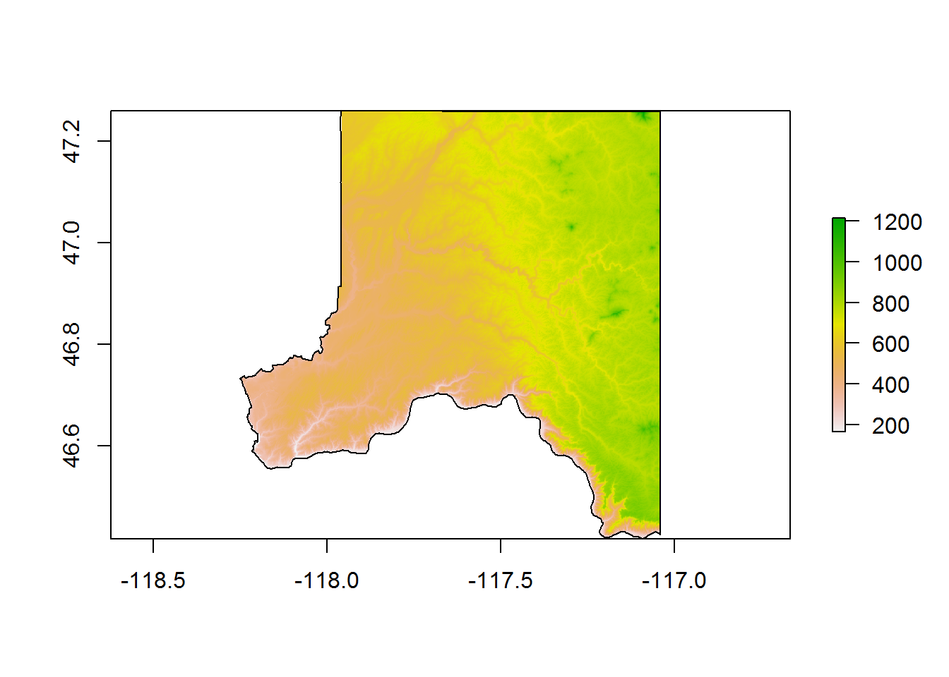
The NED elevation data was downloaded for our study area, cropped to the rectangular extent of the county, and then masked to the county.
9.8 Are sites situated based on elevation?
Alright, now that all of our data are in place, we can get to the meat of our analysis: are cell towers in especially high places in Whitman county? Here, we treat Whitman county as the decision space within which some past cellular engineers decided to build towers—our null hypothesis is that there is no relationship between elevation and cell tower location. Put another way, our task is to rule out whether cell towers were likely to have been placed randomly across the landscape. We’ll first extract the elevations for the cell towers, then calculate a probability density estimate for the cell towers, estimate a probability density curve for the landscape using Monte Carlo resampling, and finally compare the two distributions graphically and numerically using a Mann-Whitney U test.
9.8.1 Extract site elevations
Extracting the cell tower elevations is straightforward using the extract() function from the raster package.
# Extract cell tower elevations from the study area NED values

# knit in bookdown gives error with sf -> spatial, so here's a workaround
library(rgdal)
library(sp)
cell_towers_sp <- SpatialPoints(st_coordinates(cell_towers),
                                  CRS(proj4string(my_county_NED)))


cell_towers_spdf <- SpatialPointsDataFrame(cell_towers_sp, data.frame(cell_towers))


cell_towers$`Elevation (m)` <-
  raster::extract(my_county_NED,
                  cell_towers_spdf)


# cell_towers$`Elevation (m)` <-  raster::extract(my_county_NED,
#                                                as(cell_towers, "Spatial"))

cell_towers
## Simple feature collection with 41 features and 4 fields
## geometry type: POINT
## dimension: XY
## bbox: xmin: -176.6418 ymin: 13.27747 xmax: -64.68769 ymax: 71.31036
## epsg (SRID): 4326
## proj4string: +proj=longlat +datum=WGS84 +no_defs
## # A tibble: 41 × 5
## `Unique System Identifier` `Entity Name`
## <int> <chr>
## 1 597094 Qwest Corporation
## 2 597409 NORTHWEST LEASE ONE, L.L.C.
## 3 597902 SINCLAIR LEWISTON LICENSEE, LLC
## 4 598225 Inland Cellular LLC
## 5 598624 AVISTA CORPORATION
## 6 598630 AVISTA CORPORATION
## 7 599225 WASHINGTON STATE UNIVERSITY
## 8 609045 UNION PACIFIC RAILROAD
## 9 612883 PALOUSE COUNTRY INC.
## 10 2606107 Washington State University
## # ... with 31 more rows, and 3 more variables: `Height of
## # Structure` <dbl>, `Elevation (m)` <dbl>, geometry <simple_feature>9.8.2 Calculate kernel density curves for sites and landscape
We can calculate kernel density curves using the density() function available in all R installations. This code block gets a little complicated. The first section is strightforward: we estimate the probability density for all elevations between 150 and 1250 masl (the domain of the county elevation). The second section is a bit more complicated: we estimate probability densities for 99 random samples from the elevation data. (You would probably want to draw more resamples than this in a real analysis). Each sample is of the same number of sites as there are cell towers. This is called Monte Carlo resampling. The code section performs the sampling, then calculates a 95% confidence interval for the sampled data using quantiles. We will use the foreach package (and its %do% function) to repeat and output the resampling.
# Calculate the cell tower densities
# -------------------------
cell_towers_densities <- cell_towers %$%
  `Elevation (m)` %>%
  density(from = 150,
            to = 1250,
            n = 1101) %>%
    tidy() %>%
    tibble::as_tibble() %>%
  dplyr::mutate(y = y * 1101) %>%
  dplyr::rename(Elevation = x,
                Frequency = y)


# Calculate possible densities across the study area using resampling
# -------------------------
# Load the NED elevations into memory for fast resampling
my_county_NED_values <- my_county_NED %>%
  values() %>%
  na.omit() # Drop all masked (NA) locations

# Draw 99 random samples, and calculate their densities
my_county_NED_densities <- foreach::foreach(n = 1:99, .combine = rbind) %do% {
  my_county_NED_values %>%
    sample(nrow(cell_towers),
           replace = FALSE) %>%
    density(from = 150,
            to = 1250,
            n = 1101) %>%
    broom::tidy() %>%
    tibble::as_tibble() %>%
    dplyr::mutate(y = y * 1101)
} %>%
  dplyr::group_by(x) %>%
  purrr::by_slice(function(x){
    quantile(x$y, probs = c(0.025, 0.5, 0.975)) %>%
      t() %>%
      broom::tidy()
  }, .collate = "rows") %>%
  magrittr::set_names(c("Elevation", "Lower CI", "Frequency", "Upper CI"))
9.8.3 Plot the kernel density curves
We’ll perform a statistical test on the cell tower and resampled elevation data in a minute, but first it is just as helpful to view a graph of the two data sets. Like all things, R has many different ways of graphing data, but the ggplot2 package from Hadley Wickam is fast becoming the framework-du jour for graphics in R. The plotly package can be used to effortly convert ggplot2 graphs into interactive HTML graphics. ggplot2 uses a pipe-like system for building graphs, where graphical elements are appended to one-another using the + operator. Hover over the plot to explore it interactively.
# Plot both distributions using ggplot2, then create an interactive html widget using plotly.
g <- ggplot() +
  geom_line(data = my_county_NED_densities,
            mapping = aes(x = Elevation,
                          y = Frequency)) +
  geom_ribbon(data = my_county_NED_densities,
              mapping = aes(x = Elevation,
                            ymin = `Lower CI`,
                            ymax = `Upper CI`),
              alpha = 0.3) +
  geom_line(data = cell_towers_densities,
               mapping = aes(x = Elevation,
                             y = Frequency),
               color = "red")

ggplotly(g)# Create the HTML widget
This plot is revealing. The landscape data (represented by the black line and gray confidence interval) is left skewed and has two modes at c. 550 and 750 masl. In contrast, the cell tower data has a single dominant mode at c. 780 masl, and is slightly right skewed. From this visual investigation alone, we can see that the cell tower locations were unlikely to have been randomly sampled from the landscape as a whole.
9.8.4 Mann-Whitney U test comparing non-normal distributions
Because neither of these distributions are statistically normal, we will use the nonparametric Mann-Whitney U test (also known as a Wilcoxon test) to test whether the cell tower locations were likely a random sample of locations drawn from our study area. Again, we’ll use Monte Carlo resampling to generate confidence intervals for our test statistic. Finally, we will output the test data to a comma-seperated values (CSV) file for inclusion in external reports.
# Draw 999 random samples from the NED, and compute two-sample Wilcoxon tests (Mann-Whitney U tests)
my_county_Cell_MWU <- foreach(n = 1:99, .combine = rbind) %do% {
  my_county_sample <- my_county_NED_values %>%
    sample(nrow(cell_towers),
           replace = FALSE) %>%
    wilcox.test(x = cell_towers$`Elevation (m)`,
                y = .,
                alternative = "greater",
                exact = FALSE) %>%
    tidy() %>%
    tibble::as_tibble()

} %>%
  dplyr::select(statistic, p.value)

# Get the median test statistic and 95% confidence interval
my_county_Cell_MWU <- foreach::foreach(prob = c(0.025,0.5,0.975), .combine = rbind) %do% {
  my_county_Cell_MWU %>%
      dplyr::summarise_all(quantile, probs = prob)
} %>%
  t() %>%
  magrittr::set_colnames(c("Lower CI","Median","Upper CI")) %>%
  magrittr::set_rownames(c("U statistic","p-value"))

# Write output table as a CSV
my_county_Cell_MWU %T>%
  write.csv("OUTPUT/Mann_Whitney_results.csv")
## Lower CI Median Upper CI
## U statistic 1.181600e+03 1.333000e+03 1.474650e+03
## p-value 2.102591e-09 2.523619e-06 7.981066e-04The results of the Mann-Whitney U two-sample tests show that it is highly unlikely that the cell towers in Whitman county were randomly placed across the landscape (median U statistic = 1333, median p-value = 2.523619110^{-6}). We can infer from the graphical analysis above that the cell towers were placed on unusually high places across the landscape.
9.8.4.1 Conclusions
R is extremely powerful as a geo-analytic tool, and encountering sophisticated code for the first time can be daunting. But R can also be useful for basic exploratory spatial analysis, quick-and-dirty statistical testing, and interactive data presentation. I hope this short tutorial gave you a taste of how useful R can be.
9.8.5 References cited
sessionInfo()## R version 3.3.3 (2017-03-06)
## Platform: x86_64-w64-mingw32/x64 (64-bit)
## Running under: Windows 7 x64 (build 7601) Service Pack 1
##
## locale:
## [1] LC_COLLATE=English_Australia.1252 LC_CTYPE=English_Australia.1252
## [3] LC_MONETARY=English_Australia.1252 LC_NUMERIC=C
## [5] LC_TIME=English_Australia.1252
##
## attached base packages:
## [1] methods stats graphics grDevices utils datasets base
##
## other attached packages:
## [1] rgdal_1.2-5 FedData_2.4.5 htmltools_0.3.5 leaflet_1.1.0
## [5] raster_2.5-8 sp_1.2-4 sf_0.4-1 plotly_4.5.6
## [9] ggplot2_2.2.1 broom_0.4.2 tidyr_0.6.1 dplyr_0.5.0
## [13] tibble_1.2 purrr_0.2.2 foreach_1.4.3 magrittr_1.5
##
## loaded via a namespace (and not attached):
## [1] reshape2_1.4.2 lattice_0.20-34 colorspace_1.3-2
## [4] viridisLite_0.2.0 yaml_2.1.14 base64enc_0.1-3
## [7] foreign_0.8-67 DBI_0.6 plyr_1.8.4
## [10] stringr_1.2.0 rgeos_0.3-22 munsell_0.4.3
## [13] gtable_0.2.0 htmlwidgets_0.8 codetools_0.2-15
## [16] psych_1.7.3.21 evaluate_0.10 labeling_0.3
## [19] knitr_1.15.17 doParallel_1.0.10 httpuv_1.3.3
## [22] crosstalk_1.0.0 parallel_3.3.3 Rcpp_0.12.10
## [25] readr_1.1.0 xtable_1.8-2 udunits2_0.13
## [28] scales_0.4.1 backports_1.0.5 jsonlite_1.3
## [31] mime_0.5 mnormt_1.5-5 hms_0.3
## [34] digest_0.6.12 stringi_1.1.3 bookdown_0.3.16
## [37] shiny_1.0.0 ncdf4_1.15 grid_3.3.3
## [40] rprojroot_1.2 tools_3.3.3 lazyeval_0.2.0
## [43] data.table_1.10.4 lubridate_1.6.0 assertthat_0.1
## [46] rmarkdown_1.4 httr_1.2.1 iterators_1.0.8
## [49] R6_2.2.0 compiler_3.3.3 units_0.4-3
## [52] nlme_3.1-131References
Kowalewski, Stephen A. 2008. “Regional Settlement Pattern Studies.” Journal of Archaeological Research 16: 225–85.
Graves McEwan, Dorothy. 2012. “Qualitative Landscape Theories and Archaeological Predictive Modelling—A Journey Through No Man’s Land?” Journal of Archaeological Method and Theory 19: 526–47.
Kohler, Timothy A., and Sandra C. Parker. 1986. “Predictive Models for Archaeological Resource Location.” Advances in Archaeological Method and Theory 9: 397–452.
Maschner, Herbert D.G., and Jeffrey W. Stein. 1995. “Multivariate Approaches to Site Location on the Northwest Coast of North America.” Antiquity 69 (262): 61–73.
Axtell, Robert L., Joshua M. Epstein, Jeffrey S. Dean, George J. Gumerman, Alan C. Swedlund, Jason Harburger, Shubha Chakravarty, Ross Hammond, Jon Parker, and Miles Parker. 2002. “Population Growth and Collapse in a Multiagent Model of the Kayenta Anasazi in Long House Valley.” Proceedings of the National Academy of Sciences 99 (suppl 3): 7275–9.
Griffin, Arthur F., and Charles Stanish. 2007. “An Agent-Based Model of Prehistoric Settlement Patterns and Political Consolidation in the Lake Titicaca Basin of Peru and Bolivia.” Structure and Dynamics 2 (2): 1–47 [online].
Kohler, Timothy A., and Mark D. Varien, eds. 2012. Emergence and Collapse of Early Villages: Models of Central Mesa Verde Archaeology. Berkeley, California: University of California Press.
Bocinsky, R. Kyle. 2014. “Extrinsic Site Defensibility and Landscape-Based Archaeological Inference: An Example from the Northwest Coast.” Journal of Anthropological Archaeology 35: 164–76.
Martindale, Andrew, and Kisha Supernant. 2009. “Quantifying the Defensiveness of Defended Sites on the Northwest Coast of North America.” Journal of Anthropological Archaeology 28 (2): 191–204.
Sakaguchi, Takashi, Jesse Morin, and Ryan Dickie. 2010. “Defensibility of Large Prehistoric Sites in the Mid-Fraser region on the Canadian Plateau.” Journal of Archaeological Science 37 (6): 1171–85.
Johnson, C David. 2003. “Mesa Verde Region Towers: A View from Above.” Kiva 68 (4). JSTOR: 323–40.
Van Dyke, Ruth M., R. Kyle Bocinsky, Tucker Robinson, and Thomas C. Windes. 2016. “Great Houses, Shrines, and High Places: Intervisibility in the Chacoan World.” American Antiquity 81 (2): 205–30.