Chapter 4 Agent-based modelling prehistoric landscape use with R and NetLogo
Ben Davies
Built using R version 3.3.3 and NetLogo version 6.0.
4.0.1 Introduction
Where I work in western New South Wales, Australia, heat retainer hearths are a common feature of archaeological landscapes. The hearths are manifest as concentrations of fire-altered stone on the surface. Sometimes, these concentrations protect dense caps of burned sediment and charcoal, the latter of which can be used to date the hearths.
The temporal distribution of dates obtained from hearths at Rutherfords Creek show two patterns: a superlinear increase in the frequency of dates through time, and episodic gaps in the chronometric data. The increasing frequency of dates is typically explained in terms of either population growth or taphonomic loss, while the gaps are variously explained as being the result of periods of temporary abandonment, or cyclical expanasions and contractions of foraging ranges.
The visibility of these hearths, and their retention of charcoal, is largely a product of a fluvial geomorphic environment, where episodic flood move sediment around the landscape. This tutorial draws on a study aimed at understanding how the frequency of erosion and deposition affects the distribution of datable features in a surface context.
4.0.2 Agent-based modeling with NetLogo and R
This tutorial demonstrates the use of the RNetLogo package to facilitate the analysis of NetLogo agent-based models. Agent-based models are computer simulations in which individual system components (often in the form of autonomous computational “agents”) interact with each other and/or their environment according to a given set of rules. These micro-level interactions can generate macro-level regularities over time, allowing the modeller to observe the emergence of these larger patterns or entities as outcomes of smaller-scale activities.
NetLogo is a modeling environment used to build agent-basd models. NetLogo can interface directly with R in two ways: either through an extension that comes bundled with NetLogo , or through the RNetLogo package in R. Both of these were developed by Jan C. Thiele.
This tutorial uses a NetLogo model called HMODEL, aimed at understanding how the frequency of erosion and deposition affects the distribution of datable features in a surface context. Before getting started, you’ll need to make sure that you have NetLogo, R, and the RNetLogo package installed.
4.0.3 Starting NetLogo from R
First, add the RNetLogo package to your current R session:
Next, we need to tell R where to find NetLogo is stored, specifically where the NetLogo.jar file is stored. On a Windows machine, this is probably somewhere like C:\Program Files\NetLogo 6.0\app (this can be edited below to locate this file on your machine). Once the NetLogo.jar file has been located, the code will identify the directory where it is located, then start NetLogo from R.
To open a model, we need to tell R where the NetLogo file is located using the NLLoadModel function. The working directory, however, now been changed from the folder where this document is located to the folder where the NetLogo This code will open the hmodel.nlogo file by referring back to the home folder.
4.0.4 Running a NetLogo model from R
The RNetLogo extension calls out to NetLogo’s command line using the NLCommand and NLDoCommand functions. These will either perform one command, or perform them a preset number of times. So we can use NLCommand to run the setup routine and set parameters (in this case, surface stability), and we can use NLDoCommand to run the simulation for 2000 time steps (on the 2001st step, the simulation collects data).
NLCommand("Setup") #runs the NetLogo setup command
NLCommand("random-seed 4321") #sets the random number seed
NLCommand("set surface_stability 0") #sets the surface_stability parameter
NLDoCommand(2001,"Go") #runs the model for 2000 iterations
If you switch to the NetLogo GUI, you can see HMODEL operating. In the model, simulated agents move randomly from point to point within a gridded space, constructing hearths, shown as an X, at a constant rate. Hearths contain an “age” which records the date the hearth was formed in years before present. If nothing else were to happen, the record would show no change through time.
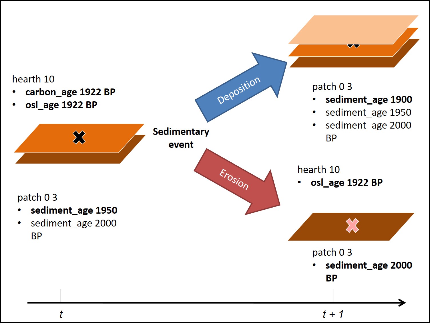
Grid cells also contain a set of sedimentary layers, each of these also containing an age, with new hearths being constructed on the surface. At a given interval, an event will occur with one of two outcomes: erosion or deposition. If erosion occurs, the top layer of sediment erodes, any hearths situated on that surface lose their charcoal and become , while surfaces underneath become visible. If deposition occurs, a layer of sediment is added to the cell, and any hearths visible on the surface become hidden and thus undetectable in a surface survey.

Diagram of HMODEL
This simulation runs from 2000 BP to present, with hearth construction ceasing at 200 BP. At the end of the simulation, we can sample the hearths sitting on the surface and compare the chronologies we obtain from them. Hearths can be dated based on radiocarbon (for hearths containing charcoal), or optically stimulated luminsence (for hearth stones). The model keeps track of all hearths above and beneath the surface, as well as the intervening stratigraphic layers, so in effect the model can be “excavated”.
4.0.5 Getting data back from NetLogo
First, we’ll use the ‘NLReport’ function to get lists of 100 randomly chosen hearths from three populations: visible hearths with charcoal that can be dated using radiocarbon, visible hearths with or without charcoal that can be dated using OSL, and the population of all hearths, visible or not. This last category should be completely unaffected by the model.
hearth_c14<- NLReport("[who] of n-of 100 hearths with [ hidden? = false and charcoal? = true ]")
hearth_osl<- NLReport("[who] of n-of 100 hearths with [ hidden? = false ]")
hearth_null<- NLReport("[who] of n-of 100 hearths")
Next, we’ll create three empty tables, or dataframes, each with columns for hearth ID number, X and Y coordinates, and hearth age in years before present.
c14_sample<-data.frame(ID=integer(),X=double(),Y=double(),age=integer())
osl_sample<-data.frame(ID=integer(),X=double(),Y=double(),age=integer())
null_sample<-data.frame(ID=integer(),X=double(),Y=double(),age=integer())
Finally, we will go through each entry in our three lists of IDs using a for loop, pull the spatial and chronometric data listed above, and populate the tables with data from the simulated hearth sample.
for (i in c(1:100)){
  c14_sample[i,]<-c(hearth_c14[i],NLReport(c(paste("[xcor] of hearth ",hearth_c14[i]),paste("[ycor] of hearth ",hearth_c14[i]),paste("[age] of hearth ",hearth_c14[i]))))
  osl_sample[i,]<-c(hearth_osl[i],NLReport(c(paste("[xcor] of hearth ",hearth_osl[i]),paste("[ycor] of hearth ",hearth_osl[i]),paste("[age] of hearth ",hearth_osl[i]))))
  null_sample[i,]<-c(hearth_null[i],NLReport(c(paste("[xcor] of hearth ",hearth_null[i]),paste("[ycor] of hearth ",hearth_null[i]),paste("[age] of hearth ",hearth_null[i]))))
}
The result should be tables for each of three populations, each containing 100 hearths, their X and Y coordinates, and their age. For those who don’t have NetLogo installed, you can simply enter the following lines to read in the same data from comma-separated value files.
c14_sample<-read.csv("c14_hearths.csv",stringsAsFactors=FALSE)
osl_sample<-read.csv("osl_hearths.csv",stringsAsFactors=FALSE)
null_sample<-read.csv("null_hearths.csv",stringsAsFactors=FALSE)
We can look at the first few entries in each table using the head function. For example:
head(c14_sample)## ID X Y age
## 1 7725 6.03502109 24.182946 456
## 2 6804 11.08510667 4.779465 641
## 3 8573 20.41160048 28.248093 287
## 4 8662 25.97655397 20.660641 269
## 5 5849 26.98930035 30.374603 832
## 6 3928 -0.07997035 29.392092 1216There is another (far simpler) way to do this using the RNetLogo extension, using the NLGetAgentSet function to obtain information from a subset of agents. For example:
c14_sample2<-NLGetAgentSet(c("who","xcor","ycor","age"),"n-of 100 hearths with [ hidden? = false and charcoal? = true]",as.data.frame=TRUE)
However, the NetLogo software has recently undergone a substantial update, and this function in the RNetLogo package has come into conflict with the new version. I’ve been in touch with developer, who assures me this is being resolved.
4.0.6 Plotting the data
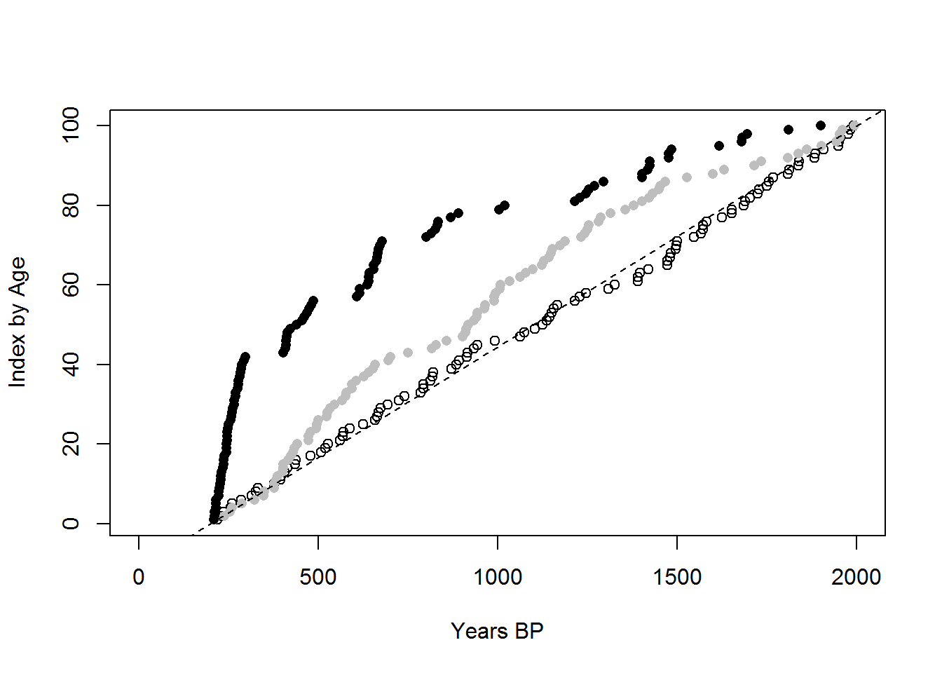
To compare, we’ll plot the ages in chronological order by age. A record weighted toward the present should bend to the left, while a record weighted toward the past should bend to the right.
plot(sort(null_sample$age),c(1:100),xlab="Years BP",ylab="Index by Age",main="",xlim=c(0,2000))
points(sort(osl_sample$age),c(1:100),pch=16,col="grey")
points(sort(c14_sample$age),c(1:100),pch=16)
abline(-11.11111111,0.055555555555555555555,lty=2)
The diagonal dashed line shows what would be expected from a uniform record between 2000 and 200 BP. What this shows is the the process as modelled can produce the patterns of increasing frequency toward the present and pronounced gaps in a radiocarbon chronology (black dots), while at the same time showing a less pronounced increase and a lack of notable gaps in the OSL chronology (grey dots). The null distribution effectively follows the dashed line, as expected (unfilled dots).
This is a point of difference from previous explanations. If the gaps in the radiocarbon record were an outcome of periodic human absence from the area, then no hearths should be constructed during the periods of absence; therefore, we should expect to see gaps in both the radiocarbon and OSL chronologies. However, the process in HMODEL can produce a chronometric record where gaps are present in the radiocarbon, but not the OSL.
When these two proxies are compared with data from the field, specifically the Rutherfords Creek study area, we can see a similar trend, where conspicuous gaps in the C14 data are absent from the OSL data, casting doubt on the notion that the gaps are the result of changes in human occupation.

Comparing C14 and OSL data (n=93) from Rutherfords Creek, New South Wales
4.0.7 Quitting NetLogo from R
In order to quit this session of NetLogo, use the NLQuit function
NLQuit()Keep in mind that once you have opened a NetLogo file using R, you are not able to open another in the same R session. You will need to restart the R session to open another model.
sessionInfo()## R version 3.3.3 (2017-03-06)
## Platform: x86_64-w64-mingw32/x64 (64-bit)
## Running under: Windows 7 x64 (build 7601) Service Pack 1
##
## locale:
## [1] LC_COLLATE=English_Australia.1252 LC_CTYPE=English_Australia.1252
## [3] LC_MONETARY=English_Australia.1252 LC_NUMERIC=C
## [5] LC_TIME=English_Australia.1252
##
## attached base packages:
## [1] methods stats graphics grDevices utils datasets base
##
## other attached packages:
## [1] RNetLogo_1.0-3 igraph_1.0.1 rJava_0.9-8
##
## loaded via a namespace (and not attached):
## [1] backports_1.0.5 bookdown_0.3.16 magrittr_1.5 rprojroot_1.2
## [5] tools_3.3.3 htmltools_0.3.5 yaml_2.1.14 Rcpp_0.12.10
## [9] stringi_1.1.3 rmarkdown_1.4 knitr_1.15.17 stringr_1.2.0
## [13] digest_0.6.12 evaluate_0.10