Chapter 2 Introduction

2.1 Overview

The goal of “Archaeological Science with R” is to give you a solid foundation into using R to do archaeological science. By archaeological science, I mean, systematic, objective, and empirical research into past human behaviours using data collected from material remains and traces. The goal is not to be exhaustive, but to instead focus on what I think are the critical skills for doing archaeological science with R. Some archaeologists already use R in an ad hoc way, for a quick plot here, or a linear model there. If you are one of these people, you will see some familiar things in this book. But you will also see a lot of new ideas, because this book will show you how R can be at the center of your entire research workflow, from when you start working with raw data until your final thesis, report, or manuscript is complete.

2.2 Why do archaeologists need to learn to code?

This book aims to solve a specific problem. The problem is that the majority of archaeologists receive little or no training in scientific programming for data analysis and visualization, and yet they routinely analyse and visualise data. A command-line interface program such as R is ideal for this kind of work, and yet is unfamiliar and exotic to most archaeologists. A command-line interface refers to interacting with software by sending instructions to the program as lines of plain text. Instead, most archaeologists use Microsoft Excel, SPSS, or similar commercial point-and-click software. There are four problems with this.

It usually results in a lot of time-consuming repetition, like copying-and-pasting between sheets in Excel, and between Excel and Microsoft Word. In recent years, biologists have seen great increases in volumes of genomic data, due to improvements in sequencing technology. This has led them to search for more efficient ways to analyse their data, and automate their analyses. They found that spreadsheet programs did not provide enough flexibility to conduct their analyses. As a result, many have turned to R, Python, and similar programming languages to overcome the limitations and inefficiencies of Excel. The key detail here is a shift from the point-and-click interface of a spreadsheet program, to the command-line interface of a programming language where we supply instructions to the computer in plain text.
It limits the development of new methods because the you are limited to what is available in the commercial software. With most commercial software packages, you are limited to the suite of functions they choose to make available to you. With an open source programming language, you and anyone else are free to implement new methods. R has extensive functions for data analysis. This includes features likes missing values and subsetting. But more importantly, R has a large set of packages (currently >10,000) for quantitative analysis, visualisation, and importing and manipulating data. For most archaeologists, whatever analysis or plot you are attempting, chances are that someone has already tried it, or something very similar, and made the code available in an R package. R is also the lingua franca for researchers in statistics, who will often publish an R package to accompany their scholarly articles. This often means immediate access to the very latest statistical techniques and implementations.
Commercial software (and even some free software) also makes it difficult to demonstrate and ensure reproducibility due to the ephemeral nature of point-and-click interfaces. Point-and-click interfaces are familiar and easy to use for most people because they are very common in software programs. But it is very challenging to efficiently record a sequence of complex clicks so that another person (or you in the future) can unambiguously repeat the procedure. This means it is difficult to make your analyses reproducible if all your work is done with a mouse. It is not practical to completely abandon using a mouse when using a computer, but by using a command-line program such as R, we can record the most important steps of the analysis workflow in plain text code. Then we have an detailed record of the steps in our analysis that we can easily share with others, and re-use ourselves, months or years into the future
Commercial software limits transparency in research because the algorithms behind the functions are not available for convenient inspection and modification. Staticians have long noted that Excel has flawed statistical procedures (McCullough and Heiser 2008, @yalta2008accuracy), and introductory texts on statistics warn students not to use Excel when the results matter (eg. Keller 2000). With an open source program such as R, you can easily inspect and alter the algorithms behind every operation. R in particular has the added advantage of being one of the most accurate software programs for statistical analysis (Almiron, Almeida, and Miranda 2009, @keeling2007comparative).

Using a command-line program such as R goes a long way towards solving these four problems.

This book is complimentary to the major textbooks and handbooks of quantitative archaeology (Baxter 2003; 1994, Van Pool and Leonard 2011, Drennan 2009, Shennan 1997). These are excellent for relevant statistical theory, discussion, and examples, and this book does not replace them on your shelf. However, those books have three limitations that we will address in the following chapters.

First is the absence of ‘plug-and-play’ examples, leading the reader to invest substantial effort to implement a method described using formulae, creating many opportunities for error. Van Pool and Leonard 2011 instruct their reader to do their statistical analyses by hand, an impractical and outmoded recommendation when computers are readily available. The amount of effort required by these texts is prohibitive to rapid exploration and experimentation of data using new methods. This book includes reproducible examples using real data sets so you can easily step-through the analysis to explore the effects of different parameters, and easily interchange your own data.
The existing books give little coverage to intuitive and methodologically more robust methods such as resampling and Bayesian analyses, favoring traditional parametric methods. This reflects a time when computational power was scarce, and computations often done by hand or with a calculator (cf Fletcher and Lock 1991). Modern computers can now easily handle resampling and Bayesian methods, and R is unique in having a mature set of methods for computing common tests in these frameworks. These methods are also increasingly common in the published research literature. This book introduces these alternative approaches to give you more options in your analytical toolkit.
The currently available books are silent on the practical mechanics of many common data analysis and visualization tasks in archaeology that are not traditionally considered statistics. This includes displaying and analyzing stratigraphic information from excavation and spatial data from surveys. Learning a tool-chain for these tasks is traditionally done on your own, and often at substantial expense with proprietary software. This book demonstrates how to write simple programs that are especially useful for archaeologists. By doing this, and providing code for other common tasks, this book addresses the need for instruction in a comprehensive open source tool-chain for these common tasks in archaeological science. It does this by presenting a reproducible research environment to show how R and its contributed packages can be used for start-to-finish research into survey, excavation, and laboratory data.

My hope is that a practical and accessible introduction to reproducible research, such as this book aims to provide, will improve openness and transparency in archaeology generally. It will contribute towards creating a community of researchers where it it normal and routine to publish code and data (after appropriate precautions are taken to protect sensitive information) with reports and publications, so that we can engage more deeply with, and learn more efficiently from, each other.

This is not a book of detailed discussions of statistical theory, and you will be referred to other texts on technical details of algorithms, etc. This is a book introducing R for practical and efficient implementations of common tasks in archaeological science, and serves as a springboard to more advanced R programming. The specific topics covered in this book are:

Implementing reproducible research with literate programming as a practice that is good for science generally, and good for your individual productivity
Working with common archaeological data structures, ingesting them into R and manipulating them from messy formats to tidy formats ready for analysis
Working with data from stone artefacts, faunal remains, pottery, glass, and metal artefacts
Compositional analysis using cluster and principle components analyses of multivariate data
Working with relative and absolute chronologies by doing seriation, and calibrating, analysing and visualising radiocarbon dates
Visualising and analysing stratigraphic data from archaeological excavation
Visualising spatial data by making maps, doing spatial analysis and site classification
Simplifying collaborative research with version control

2.3 Why R?

If you are new to R, you might wonder what the appeal is, especially when there are so many programs and languages in common use. Some of the characteristics that drew me to learn R include:

It’s free, open source, and available on every major type of computer. As a result, if you do your analysis in R, there is a very good chance that anyone with a computer can easily reproduce it. You do not have to purchase a license or subscription to use R.
It is specialised for use with statistical analysis and data visualisation. R was originaly develped by statisticians, and continues to be widely used by professional and academic statisticians. This means that there are strong links between the statistical literature and R code. Many of its algorithms have been vetted by publication and thoroughly tested through extensive use. It is easy to go from statistical theory to practice using R.
An active, supportive and generally progressive community. It is easy to get help from experts on the internet. You can also connect with other R learners via social media, and through many local user groups. I have found Stack Overflow (more on this below) and twitter to be particularly useful sources of information. Package authors are often pleased to see their packages used by others, and willing to answer questions about your use of their package.
Flexible tools for communicating your results. R packages make it easy to produce html, pdf, or Microsoft Word documents that include text, tables and figures, all generated from R code. I find this to be a substantial time-saver, especially when weeks or months pass between working on a project, and I cannot remember all the details of the last work I did. When I look over my R code I can quickly recall my analysis plan and resume from where I stopped.

2.4 Who should read this book

This book is written for archaeologists who are keen to expand their analytical horizons and gain access to new methods and more efficient ways of organising their research process. No prior knowledge about R, computer science or programming is expected, but a curiosity about statistics would be an advantage, as well as a readiness to read beyond this book to make decisions about the suitability of statistical methods for your specific research questions.

This book is intended for readers looking for practical applications of R for archaeological science. For general-purpose, gentle introductions to R, take a look at De Vries and Meys (2015) and Braun and Murdoch (2016). If you have some programming experience, and are looking for a more comprehemsive introduction to the R language, I recommend Matloff (2011) and Wickham (2014).

Most of the methods presented here are foused on rectangular data, that is, data that are typically entered into spreadsheet and database files. More specifically, the book is aimed at archaeolgists using data that is organised into rows (i.e. variables) and columns (i.e. specimens, samples or observations). There are lots of archaeological datasets that are organised differently, such as images and text. Although R is also useful for those, we do not discuss them in detail here. Rectuangular data are very common in archaeology, and many other fields, so that is why we concentrate on those here.

This book is useful for archaeologists working with small data (i.e. < 1 million rows, < 2 Gb per file) that can be stored on your computer (rather than a remote data appliance). In my experience, the majority of archaeologists work with data at this scale, so the methods presented here will be useful for the majority of archaeological applications. If your data are bigger than this, you are probably doing something very specialised and will have unique challenges to make your research reproducible. However, you can still use R and the methods decribed here for working on subsets of your large dataset.

2.5 Prerequisites

To run the code in this book, you will need to have R installed on your computer, as well as RStudio, an application that makes it substantially easier to use R. Although I have been interested in R for many years, it was only after RStudio was first released that R replaced Excel and SPSS for me. Both R and RStudio are free to download and easy to install. You can install it on most recent versions of Windows, OSX (Mac) or Linux. When used together, R and RStudio will help you to have a smooth and efficient experience when programming. RStudio provides many features that greatly simplify programming with R (my favourite is tab-completion). I do not recommend using R without RStudio, especially for the beginner.

You should download and install both R and RStudio before attempting to follow any of the examples in this book. If you have installed these programs on your computer in the past, you should update them now (new versions of R are released every six months).

2.5.1 R

To install R, visit cran.r-project.org. CRAN is the ‘Comprehensive R Archive Network’ which hosts the official releases of the R software and documentation. Then click the link that matches your operating system. What you do next will depend on your operating system. You will need to install a development environment, this is also specific to your operating system. The development environment provides some additional programs that give you access to more advanced features of the R language. The examples in this book have been tested to work in R version 3.6.0 (2019-04-26), and may not work in earlier versions.

Here’s a summary of the basic steps to download and install R for common operating systems:

Mac users should click the most current release. This will be the .pkg file at the top of the page. Once the file is downloaded, double click it to open an R installer. Follow the directions in the installer to install R. You should also install Xcode from the Mac App Store to install the development environment.
Windows users should click “base” and then download the most current version of R, which will be linked at the top of the page. You should also install Rtools to install the development environment.
Linux users will need to select their distribution and then follow the distribution specific instructions to install R. cran.r-project.org includes these instructions along side of the files to download.

If you are not sure about these download and install steps then you should research the general methods of installing software for your operating system (e.g. how-to videos on youtube), which are beyond the scope of this book.

After installing R on your computer, you may be tempted to open it and start exploring. I don’t recommend this because the R user interface is not intuitive for novices. Instead, continue reading below about downloading and installing RStudio. Then start your explorations in RStudio, which has a more user-friendly interface.

2.5.2 RStudio

Once you have R installed, it is time to download RStudio. To download RStudio, visit www.rstudio.com/download.

Choose the installer that matches your operating system. Then click the link to download the application. Once you have the application downloaded, installation is the same as for most programs on your computer. Once RStudio is installed, open it as you would open any other application. It should look something like this:

knitr::include_graphics("images/RStudio_first_view.jpg")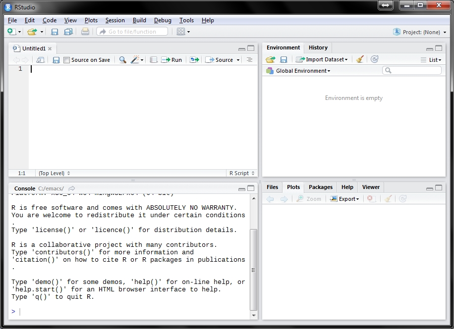

Figure 2.1: A first view of RStudio.

When you start RStudio for the first time, you’ll see your screen divided into three or four window panes. If you don’t see four window panes similar to the image above, go to File -> New File -> R Script to open a new R script file and show all four panes. One setting that is very important to change before doing any work in RStudio is how .RData files are handled. An .RData file can store the data and functions that you create in each R work session. By default, RStudio automatically saves this file when you exit RStudio, and reloads it when you start RStudio. I have only ever found this to be a source of problems and confusion. This is because it can result in temporary objects that were created during brief experiments and explorations lingering across multiple sessions as they are automatically reloaded, contaminating the workspace. So I recommend you change this default by going to the ‘Tools’ drop-down menu, select ‘Global Options…’, look in the ‘General’ section and making two changes. The first change is to uncheck ‘Restore .RData into workspace at startup’, and the second change is at the item ‘Save workspace to .RData on exit’, you should select ‘Never’. Changing these two settings will save a lot trouble as you learn how to use R’s environment, and help you to take control of the data and functionsthat you make with R. In most cases it is simplest and most efficient to treat the code that you write as the most important product while you work on analysis, and write code to export (or save) only the most important results (for example some tabular output as CSV files, and plots as PNG files), rather than automatically saving the entire workspace and all ther intermediate objects that you create along the way.

knitr::include_graphics("images/rstudio_never_restore.png")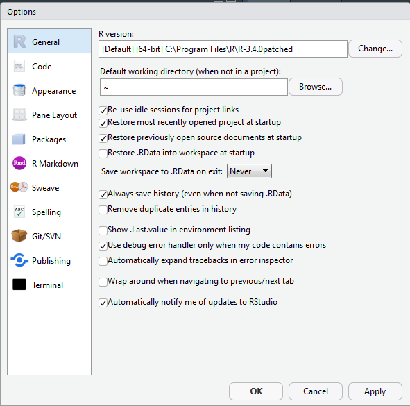

Figure 2.2: An important setting to change before using RStudio.

Here is an explanation of what you see in Figure ??. For more details about the RStudio interface, see the RStudio website https://www.rstudio.com/products/rstudio, Verzani (2011), Gandrud (2015), and Racine (2012):

The top left pane is the text editor, known as the ‘source’. This is where you write and edit code and text. The text editor in RStudio is analogus to a word processor such as Microsoft Word, but has many additional convienent features for writing and editing code. Writing code means writing in plain text, there is no bold, underline, italics or other formatting. In Chapter XX we will discuss how we can produce nicely formatted text in Microsoft Word documents using this text editor and the Rmarkdown document preparation system. We can modify the appearance of the text editor in RStudio by going to the ‘Tools’ drop-down menu, and selecting ‘Global Options…’, then browsing the options in the ‘Code’ and ‘Appearance’ sections on the left side list. I find it useful to show whitespace characters (in the Code section, Display tab), and check all the completion and diagnostic options (Code section Completeion tab and Diagnostics tabs). The code in the text editor is the most important product of your work in RStudio, so it’s a good idea to save it in a sensible place, with a meaningful name (usually R code files end in .R, with a capital R after the period), and to save it frequently while you’re working on it to minimise the risk of accidental loss.
The top right pane can have several tabs, depending on what you are doing. Most of the time you will see an ‘Environment’ tab and a ‘History’ tab. The Environment tab lists the objects that are currently available in your R session. The ‘environment’ is the place where R stores the results of calculations and functions. For example, if you have executed code that reads an Excel spreadsheet into R and stores it as an R object, then you will see this object listed in the Environment tab. This tab is useful because you can get basic information at a glance about the size of objects that you make (e.g. how many rows and columns). This is convienent for quickly checking the output of your computations so you can see if your code is working as expected. The environment is an important aspect of R because it gives us a coherent and flexible system for creating, combining and manipulating different types of data during our analysis. Environments are an advanced programming concept, and all we need to do here is note that they are helpful, and that there is nothing comparable to them in spreadsheet programs.

The History tab shows the code you have previously executed in your R session. I rarely use this tab because I write code into the text editor and save the code to my computer, so I always have a copy of the code in the text editor. I strongly recommend saving your code in a .R file for even the briefest analyses and experiments. But if you are working in an expedient fashion without saving, you can use the History tab to browse your previous commands to reuse and edit. You can also save the history of your R commands to a text file, but I don’t recommend this as it is not an efficient method for keeping track of your work. A better strategy is to write code in the text editor, interspersed with comments (lines of text prefaced with the # character) that explains what the code is doing, and save that document to your computer. We’ll discuss this strategy more in chapter XX.
The lower right pane is another multi-tab pane where plots appear, the most important are the Plots tab and the Files tab. The Plots tab allows you to conveniently browse the plots that you produce. You can navigate back to previous plots created in your current session, and interact with plots by zooming and, in some cases selecting, rotating, etc. The Plots tab has an ‘Export’ button to easily save your plots as image files on your computer (in a variety of formats), or copy to your clipboard for a quick copy-paste transfer. These are useful features for exploring pictures of your data and iterating towards a publication-quality plot.
The lower left pane is the console where code is executed. There are no buttons specific to the console, so direct interaction with this pane is limited. The most important part of this pane is the prompt, which looks like this >, and when this pane is active, there is a blinking cursor at the prompt. The space where the cursor is in is called the command line, where you type, paste, or send code. When you type at the prompt and press Enter, you are submitting code to be interpreted by R, and R will usually return the result in the console. Here is one of the simplest possible examples of using the console:

> # this is a line of text, indicated by the initial # character, it is ignored by R
> 1 + 1 # I typed 1 + 1 in the console and then pressed the 'enter' key on my keyboard
[1] 2

In this example, I placed my cursor at the prompt, typed 1 + 1 in my RStudio conosole with my keyboard, and then pressed Enter. The R interpretor returned the result, 2, directly below my input. The [1] with the square brackets indicates that this is the first item returned by the interpretor. At first glance, this [1] might seem unessecary, but this indexing is helpful when working with more complex calculations that produce more extensive output. Most of the time you wont type directly at the prompt because it is not efficient for more complex code. Instead, you’ll type code in the text editor, and send that code from the text editor to the prompt by pressing the Control + Enter keys simutanteously (on OSX: Command + Enter).

There are two useful features of the console that will save you time when working with R. First is the up arrow key on your keyboard, which allows you to re-run previous commands. If you place your cursor at the prompt, and press the up arrow key, you can browse the previously executed lines of code. Once you find the code you want to re-run, you can edit it in the console, if you wish, or simply press Enter to send it to the interpreter. The second handy feature of the console pane in RStudio is the small arrow icon at the right side of the title bar of the console. If you look at the top of the console pane, you’ll see the word “Console”, then you’ll see a path to a folder on your computer, then at the end of that, you’ll see a little curved arrow icon pointing to the right. The path on your computer in this console title bar is your ‘Working Directory’. If you click on the small arrow, it will switch the Files pane to show the contents of your Working Directory.

The Working Directory is an important concept to understand because it is unlike anything you might have seen in Excel or other point-and-click software. The Working Directory is the directory (or folder) on your computer where R is currently working. It is the location on your computer where R will look when you read files into R, or save output from R to your computer. By default, your R working directory was probably set to an inconvienent directory when you installed R (this is always the case for me), but this is easily changed. The simplest method is to go to the RStudio toolbar menu, click on ‘Session’, then ‘Set Working Directory’ then ‘To Source File Location’. You may see in other people using R code to set the working directory (setwd()), but I don’t recommend this. If you use code to set the working directory, your code will only work on your computer, in its current configuration of files and folders. This means that your code is not portable and not robust to change. If you reorganise your files, or give your code to a collaborator, the actual working directory whre your files are will no longer match what is written in the code. This can lead to errors and frustration. So while the concept of the Working Directory is important to know about for working with R, you should not include it in your R code. You may need your code to refer to other directories relative to your main project directory (for example, a directory called ‘data’ that contains spreadsheets, etc.), but that is a different task to setting the Working Directory, and we’ll look into that in Chapter XX.

Although I have described the default appearance, the location and combination of panes and tabs in RStudio are customisable via the toolbar menu (Tools -> Global Options -> Pane Layout). For example, I prefer to have to console on the upper right, and I often minimize some of the panes so I only see the text editor and the console. This makes it easier for me to keep track of what I’m doing and I don’t get distracted by unnecesary details on my screen. I also like to the use the PragmataPro font with RStudio because it I find it easier to read code in this font compared to many others.

2.6 Key terms to understand (don’t skip this bit!)

Now we’ve established the basic motivation for learning R to do archaeology, and introduced the layout of the software, we should introduce some key terms and conventions that appear frequently in this book. Becoming familiar with these terms will help you with the basic tasks of finding your way around when starting to use R.

We have already discussed the prompt and command line in the previous section, and we’ve used the word code, but without really defining it. Code refers to anything written in a programming language, from a single word to a function with thousands of lines. Code often contains comments, which you can recognise in the R language by a # symbol at the start of the line. Code comments are important because they help you and other people understand the purpose of the code. The # symbol tells the R interpretor to ignore to everything to the right of that symbol, and skip to the next line of code. There are no strict rules on how many comments your should include with your code, but a good starting point would be one line of comment for each 10 lines or major section of code. More generally, your comments should try to tell you what you need to know a few weeks or months from now when you return to work on the code after a break, and can’t recall the minutae of your previous code. A script is a file that contains code, and R script file names ends with .R. You can open these files in any program that edits text, for example Notepad on Windows (or Notepad++) or TextEdit on OSX (or Sublime Text).

A function refers to a group of code that carries out instructions to do useful work. For example, the function mean() computes the mean, or average, of a set of numbers. In this book you will always be able to recognise a function because they will always be followed by a pair of parentheses, often with code in between the parentheses. A function is a efficient way to organise code, because a single function can cause hundreds of lines of code to run to produce a result. Rather than running those hundreds of lines, one-by-one, over and over, we can simply type the function name that invokes them, and save ourself a lot of typing. Minimising typing is good because it saves time, and lowers the chances that we might introduce errors into our analysis by making typing mistakes.

Usually we want to save the output of a function so we can use it in other calculations, for plotting, or to share with our colleagues. For example, we might want to compute the mean of the lengths of an assemblage of artefacts. To keep the results of function, we assign the output to an object, this process of assignment saves the output in our environment so it is available for reuse later in our session. Assignment does not save data to a file that can be used elswhere, such as emailed as an attachment, that is a separate process called ‘exporting’ data from R which we’ll cover later. This example demonstrates the use of two simple functions to compute a mean value:

x <- c(4, 7, 12) # length measurements of three artefacts
y <- mean(x)     # compute the mean length

The c() is a function to combine (‘c’ is for combine) our artefact measuremens into a type of set called a vector. A vector is a single sequence of data elements of the same type. In our example above all elements are numbers (as in our example above). There are two other commonly used vectors in R: a character vector where all elements could be letters or words, and a logical vector where all elements are logical constants, either TRUE or FALSE. The vector is a fundamental data type in R that we will use very often. In the above example we have stored the result of the c() function in an object that we call x (we can call it almost anything that we like, and we do not need to create x in advance). The second line of code in the above example computes the mean of 4, 7, and 12 (ie. (4 + 7 + 12)/3), and then assigns, or stores, the result in a object called y. We can then use both x and y later in our workflow for other tasks. This is useful because it means we don’t have to recompute the mean repeatedly.

An important new concept in this example is the assignment operator, <-, which we can translate as ‘put the results from the right side of this symbol into the thing on the left side’. Note that in the above example I have not included the prompt character (>). Omitting this character makes it easier for you to copy and paste from this book into your R console so you can run the code yourself, and explore what happens when you make minor changes.

There’s a lot more vocabularly to come, but these are the key terms that you need to know to make sense of the rest of this book and to get started exploring R by yourself.

2.6.1 Packages

Functions, such as c() and mean() in the above example, are at the heart of working with R, and are part of the reason for R’s great versatility. They save a lot of time by minimizing typing and copy-and-pasting, so it’s worth to invest some effort into learning how to use functions, and how to write your own functions (more on that in Chapter XX). Functions are typically organised into packages, which you can download to extend the usefulness of R. We will use packages extensively in this book, and briefly discuss how and why you might write your own packages in Chapter XX.

The most common way to install R packages is to run the function, install.packages() at the R prompt. For example, if you run install.packages("binford"), you will automatically download the package binford from the repository at cran.r-project.org (you need to be connected to the internet) and install them in your system library. The binford package contains datasents from his 2001 book ‘Constructing Frames of Reference: An Analytical Method for Archaeological Theory Building Using Ethnographic and Environmental Data Sets’.

Try this yourself by opening RStudio and running these commands to install some useful packages that we will use in later chapters. You only need to use install.packages() once (per computer) to download the package files. You don’t need to do this each time you open RStudio, but to ensure you have the lastest versions of the package you might want to run update.packages() every few months. Notice how we use the c() function here to create a character vector of package names for the install.packages() function to work on:

# install a single package
install.packages("devtools")

# install multiple packages at one time
install.packages(c("dplyr", "ggplot2", 
                   "knitr", "readr", "rmarkdown", 
                   "scales", "stringr", "tidyr"))

Most of this book uses packages from a group called the ‘tidyverse’, which can be installed altogher with install.packages(tidyverse). However, I prefer to mention the individual packages by name so you have a clearer understanding of where to look to get help on specific functions, and to help you discover related functions.

Most of the packages we will use in this book are stored on cran.r-project.org, an repository maintained by a small group of expert R programmers. Other online repositories for R packages include Bioconductor, focusing on genetics software, also maintained by expert R programmers, and www.github.com, a free code-sharing website that where anyone can share their packages (without maintainers like CRAN and Bioconductor).

You can install packages stored on GitHub with the install_github() function in the devtools package (which we installed using the commands above). To use the install_github() function, pass it a character string with the form "<github username>/<github repository name>". For example, we can install the package ggbiplot to plot the output of a Principle Components Analysis like this:

devtools::install_github("vqv/ggbiplot")
# The two colons are a short-cut to avoid typing library(devtools)

When R installs a package, it downloads the package to your system library. You must use the library() function to make the contents of the package available to your current R session. Each time you open RStudio you will need to run library() to use functions in packages you have previously installed. It’s good practice to have the library() functions among the first few lines of your code for a project, so other users can quickly see what packages they will need to have to prepare to run your code. For example, to use the functions in the dplyr package, you would need to first run

library("dplyr")

You will need to rerun this library() command each time you open a new R session that uses functions from the dplyr package.

One of the strengths of R, the vibrant community of researcher-developers, is also one of its weaknesses. This is because it means that some packages are updated frequently, and others are not. Sometimes these updates can change how your code works, or stop it from working altogether. We’ll discuss some detailed solutions to this in Chapter XX. For now we’ll just note that it’s good practice to include the output of sessionInfo() in the results of your analysi because this tells you the specific version numbers for all the packakges used in your your analysis. This means that if there are breaking changes in some of the packages you’re using over the life of your project, you have a record of the last version of the packages that worked for you. You can install older versions of packages from CRAN using devtools::install_version().

2.7 Getting help

Developing fluency in a language like German or Chinese takes time, practice, and has ups and downs. Learning a programming language like R is a similar process, and you should anticipate ups and downs as R becomes an increasingly central part of your workflow. R comes with extensive built-in documentation, which is highly structured and very often contains example code that you can can run to explore how a function works. I find these runnable examples to be most useful part of the built-in documentation. You can access the built-in doucmentation with one of the following methods, which are run in the R console:

?mean                  # opens the help page for the mean function
?"+"                   # opens the help page for addition
?"if"                  # opens the help page for if
??plotting             # searches for topics containing words like "plotting"
??"regression model"   # searches for topics containing phrases like this

These methods of getting help do not require an internet connection, and so are still useful when you are offline. If you are online, here are a number of additional options for seeking help when you get stuck, or have a question. The simplest case is when you execute a line of code, only to get a cryptic error message in the console. A good first reponse is to copy the text of the error message to your clipboard, and paste it into a Google search box in your web browser. In most cases, the top search results will be from Stack Overflow or one of the R mailing lists. Sometimes this will get you a quick solution. However, sometimes error messages are too generic, or too specific, and you can browse through many pages of search results without getting any useful ideas to solve your problem. When that happens, there are a few places online where you can give some more detail about your problem, and often get helpful responses.

Stack Overflow is a free question-and-answer website that is focused on computer programming. Participants receive points for asking clear questions, and for giving useful answers. This adds a competitive element to participating in the Q&A, and when you ask a well-formed question, several answers can appear very quickly from participants eager to earn points by being the best answer to your question (you award these points, as the question-asker). The R mailing lists are more traditional email-based fora, with archives at several places online. Highly skilled R programmers and R-using scientists from a variety of disciplines are active on both the R mailing lists and Stack Overflow. I prefer Stack Overflow because responses to my questions typically come quicker, and I find it easier to see when someone else’s question has been answered, compared to browsing the email list archives.

I find that in the course of writing my question to submit to Stack Overflow, the process of simplifying my code into a small, self-contained example (a vital ingredient of a good question) leads me to discover the cause of my problem. Very often it’s as simple as a misplaced comma or bracket. Then I can answer my question before posting it and seeking help from others. Similarly, I often find that many of my questions have already been asked and answered on Stack Overflow. One of the big challenges in getting the most out of Stack Overflow and email list archives is to recognise how similar an existing question is to your current problem, and thus how useful the answers are to your specific issue.

If you are sure that your problem is new and unique, and you want to submit a question, here is some general advice to help you get a useful answer quickly, and have a pleasant experience at the same time, from the Stack Overflow and R mailing lists communities:

Spend some time browsing previous posts to understand the community norms. Online communities have specific cultural values that are often strongly held. While some of these are spelled out in posting guides, many are also unwritten, and can only be learnt through mindful reading of previous correspondence. If you are familiar with the norms, you are more likely to have an efficient and satisfying interaction with the community.
Make sure your computer has the latest version of R and of the package (or packages) you are having problems with. It may be that your problem is the result of a recently fixed bug.
Spend some time creating a simple reproducible example that captures the essence of your problem. This mean a simplified version of your problem that another person can copy and paste from their browser into their R console to reproduce the error that you see. This can be quite an art-form, but the basic ingredients for a good reproducible example are:

The packages you are using, e.g. library(dplyr)
A small data set. R comes with many example data sets built-in, if you run data() you can see a list. These are very convenient to use for reproducible examples because you can count on everyone having them. If you want to include your own data, you can use dput() to generate R code that another person can copy and paste to recreate your data set.
Code. Your code should be easy to read, with spaces between operators (+, -, *, etc.) and after commas, and conformant to a style guide, such as Hadley Wickham’s (2014) style guide in Advanced R. Your code should includes lines of commentary, which begin with #, to help others understand your problem. There should be just enough code to demonstrate your problem, don’t burden your audience with haaving to make sense of lots of your code that is not central to your question.
A description of your R environment. The usual way to communicate your R environment (ie. your operating system type and version), is to include the output from sessionInfo() or devtools::session_info() (same output, but in a tidyer format) into your question.

The reprex package by Jenny Bryan provides some convenient functions that greatly simplify this process of preparing reproducible examples for seeking help online.

Don’t worry if some of these terms are unfamiliar at the moment. The main thing to know at this point is that help is available, and that the quality of help you receive is often directly proportional to the effort you spend seeking it.

2.7.1 Draft TOC

References

Almiron, Marcelo G., Eliana S. Almeida, and Marcio N. Miranda. 2009. “The Reliability of Statistical Functions in Four Software Packages Freely Used in Numerical Computation.” Braz. J. Probab. Stat. 23 (2). Brazilian Statistical Association: 107–19. https://doi.org/10.1214/08-BJPS017.

Braun, W John, and Duncan J Murdoch. 2016. A First Course in Statistical Programming with R. Cambridge University Press.

De Vries, Andrie, and Joris Meys. 2015. R for Dummies. John Wiley & Sons.

Gandrud, Christopher. 2015. Reproducible Research with R and R Studio, Second Edition. 2nd ed. Chapman and Hall Crc the R Series. Chapman; Hall CRC. http://gen.lib.rus.ec/book/index.php?md5=89E3848976A5DFAC000A892AA29FFE8D.

Keller, Gerald. 2000. Applied Statistics with Microsoft Excel. Duxbury.

Matloff, Norman. 2011. The Art of R Programming: A Tour of Statistical Software Design. Book. No Starch Press.

McCullough, Bruce D, and David A Heiser. 2008. “On the Accuracy of Statistical Procedures in Microsoft Excel 2007.” Computational Statistics & Data Analysis 52 (10). Elsevier: 4570–8.

Racine, Jeffrey S. 2012. “RStudio: A Platform-Independent Ide for R and Sweave.” Journal of Applied Econometrics 27 (1). Wiley Online Library: 167–72.

Verzani, John. 2011. Getting Started with Rstudio. " O’Reilly Media, Inc.".

Wickham, Hadley. 2014. Advanced R. CRC Press.