Chapter 4 Collecting & organising data to analyse with R
4.1 Overview
The purpose of this chapter is to explain how thoughtful decisions made before and during the point of data collection can save time and effort later during the data analysis and visualisation process, using R or any other tool. The chapter is organised hierarchically, starting with file oranisation at the project level, then moving down to discuss efficient organisation of spreadsheets (as one of the most common tools for collecting, sharing and storing archaeological data), and finally at the highly granular level of the individual cell within a spreadsheet.
Saving time and effort is of course an important motivation for changing your data collection and analysis behaviours, however there is a greater vision that relates to data organisation principles. This vision is two-fold. First is enhancing the reproducibility of archaeological research. When a project is well-organised, it is easier to find the key files to check the previous results. Second is large-scale inter-operability of datasets, so that archaeological data from diverse projects might be easily combined to address questions that no single project can by itself. This vision has many other dependencies, such as a willingness to share data and make it publicly available, and agreement about what to measure and how to name variables. While sharing your data is the first step in allowing reuse, and this is not yet common in archaeology, to ensure that it is easy for others to reuse your data they must be easy to understand (White et al. 2013).
Much of the content of this chapter is not highly sophisticated, and might seem like common sense. However, because the practices decsribed here make a big difference to the reusability of data, I think it is important to discuss these issues directly and explicitly as part of learning about the data analysis process, rather than assume archaeologists will ‘pick them up’ along the way without any specific guidance or instruction. This chapter draws on materials in the public domain that were originally prepared by Jenny Bryan, Karl Broman, and others for Data Carpentry’s reproducible science curriculum as well as sources from other disciplines such as Borer et al. (2009), Sutter et al. (2015), Volk, Lucero, and Barnas (2014), Hampton et al. (2013), Strasser and Hampton (2012).
4.2 File organisation
4.2.1 Guidelines for organising your files for improved reproducibility
The most fundamental principle to follow to improve file organisation is simply to have a strategy and be faithful to it. A key motivation for organising files is to make it easy to work with them, both during the time of your anlaysis, and in the future when you or other people use the files. If your files are well-organised, someone unfamiliar with your project (which could also be you in the future) should be able to look at your files and quickly understand in detail what you did and why (Noble 2009). A second motivation for being organised is that for almost everything you do during your analysis, you will probably have to do it again. We commonly explore many analytical options with our data, so the process of data analysis is more like a branching tree than a single sequence of consecutive actions. Often we loop back to an earlier stage in the analysis to explore the effect of adjusting a selection of data, or the parameters of a model. This means that many parts of our analysese are redone in the natural flow of working on a project. If we have organized and documented our work clearly, then repeating the earlier steps of the analysis with minor variations will be much easier.
Beyond the fundamental principle of simply having a strategy, there are several guidelines that have been proposed by biologists and ecologists that are applicable to archaeological research (Noble 2009; White et al. 2013). These guidelines relfect the principle that file organization should indicate inputs and outputs and the flow of information during your data anlysis. The most important of these are that (1) raw data is kept separate from derived data, and (2) data is kept separate from code.
Raw data means data files as they were when you originally received them, for example transcribed from a notebook, directly entered into a database or spreadsheet, or downloaded from an instrument such as a total station or XRF. Derived data refers to the data that result from actions you take after you receive the data files. This includes manual manipulations, such as edits in an Excel spreadsheet, and programmatic manipulations that occur when you use R code to output an updated version of your data. Manual manipulations should be avoided as much as possible because they leave no trace, unlike a manipulation performed by code, making them difficult to undo if you change your mind. If a manual manipulations are necessary in your data, you should keep a plain text file with the data file and type in that file a brief narrative of the changes you make so that you have a record of them. A simple way to keep raw data separate from derived data is to have a folder (also known as a directory) called data/ that contains two directories, raw_data/ and clean_data/, see the schematic below. Using a simple structure like means you only need one copy of the original raw data files in your project files, rather than duplicating them across your file structure, which can be a source of substantial confusion about which file is the correct one.
|- data            # raw and primary data, are not changed once created
|  |- raw_data/    # raw data files, will not be altered ever
|  +- clean_data/  # cleaned data files, will not be altered once created
This practice of keeping the raw data isolated from everything else means that you are always able to loop back to the first steps of your anaysis where you read in the raw data in case you need to explore a different path or check your results. This is vital for ensuring the reproducibility of your research, and for peace of mind that you can check your results. If you make many changes to your raw data files along the way of your analysis, you may never be able to retrace your steps back to the start of your analysis, you will not have the option of checking your results, and your work will be irreproducible. Keeping the raw data intact also gives other researchers more options when they reuse your data, increasing the value of your work to the broader research community of archaeologists.
The second file organisation guidelines we can take from biologists and ecologists is closely related: data is kept separate from code. When working with an Excel file this is a very unnatural way to work. In an Excel sheet, the formulas that compute on the data are located directly adjacent to the cells that contains the data (e.g. in the rows to the right or below the data). While this may be convienent for working quickly with small tables of data, it results in a workflow where it is difficult distinguish between raw and derived data, and between data and methods (i.e. functions in speadsheet cells). This mingling of data and method is a major impediment to reproducbility and openness because the sequence of decisions made about how to analyse and visualise the data is not explicit.
Your code will change frequently while you work on an analysis, but your raw data should not change. If you keep these files in separate folders you will be less tempted to change the raw data by hand while you are writing code. This is a core principle of software design, and helps to minimise confusion when browsing the files in a project. A second reason why it is good practice to keep code separete from data is that you may be unable to share your raw data (for example, it may contain senstive information about archaeological site locations), but you may be willing to share your code. When these two compoenents of the project are well-separated, it is easy to control what can be made public and what must remain private. Here is an example of a project folder structure that shows how code and data can be seperated:
|- data/           # raw and primary data, are not changed once created
|  |- raw_data/    # raw data files, will not be altered ever
|  +- clean_data/  # cleaned data files, will not be altered once created
|
|- code/           # any programmatic code, e.g. R script files
A third guideline relating to the general idea of separation is to keep the files associated with mansuscript or report production separate from everything else. In the example below this is represented by the paper/ directory. It contains one (or more) R Markdown files that document the analysis in executable form. This means that it should be possible to render the R Markdown document into a HTML/PDF/Word file that shows the main methods, decisions and results of the analysis. This R Markdown file might connection to the code in the code/ directory by using the source function to import code from a script in code/ into the R Markdown file. This example also shows how files for tables, figures and other images can be organised:
|- data/           # raw and primary data, are not changed once created
|  |- raw_data/    # raw data files, will not be altered ever
|  +- clean_data/  # cleaned data files, will not be altered once created
|
|- code/           # any programmatic code, e.g. R script files
|
|- paper/          # all output from workflows and analyses
|  |  report.Rmd   # One or more R Markdown files
|  |- tables/      # text version of tables to be rendered with kable in R
|  |- figures/     # plots, likely designated for manuscript figures
|  +- pictures/    # diagrams, images, and other non-graph graphics
A final guideline related to the general theme of separation is to have a ‘scratch’ directory for experimentation. This directory should hold snippets of code and output that are produced during short journeys down alternative paths of the analysis, when you want to explore some ideas, but you are not sure if they will be relevant to the main analysis. If the experimental analyisis proved worthwhile, you can then incroporate it into the appropriate place in the main project folders. If the experiment is not directly relevant to the main analysis, you canleave it in the scratch directory or delete it. The most important details about the scratch directory is that everything in the this directory may be deleted at any time without any negative consequences for your project. I typically delete my scratch folder after my paper is submitted or published.
A final guideline, not related to separation, is to include a plain text file named ‘README’ (e.g. “README.txt” or “README.md”) at the top level of a project file structure to document some basic details about the project. This might include about dozen lines of text providing the project name, the names of the people involved, a brief description of the project, and a brief summary of the contents of the folders in the project. You may also wish to include similar README files in other folders in your project, for example to document instrument parameters that are important for using the raw data. Below is an example of a project file structure that includes a scratch directory and a README file:
|- data/           # raw and primary data, are not changed once created
|  |- raw_data/    # raw data files, will not be altered ever
|  +- clean_data/  # cleaned data files, will not be altered once created
|
|- code/           # any programmatic code, e.g. R script files
|
|- paper/          # all output from workflows and analyses
|  |  report.Rmd   # One or more R Markdown files
|  |- tables/      # text version of tables to be rendered with kable in R
|  |- figures/     # plots, likely designated for manuscript figures
|  +- pictures/    # diagrams, images, and other non-graph graphics
|
|- scratch/        # temporary files that can be safely deleted
|
|- README.txt     # the top level description of he project & its content
These guidelines about separation are broadly applicable to most archaeology projects, regardless of scale or methods. Some adjustments of the details provided in the schematic above may be required for large or secure datasets that cannot be stored on a laptop, and for time-consuming computations. In any case, the general principle of separation remains a useful starting point for organising files.
4.2.2 Guidelines for naming your files to improve reproducibility
As archaeologists we are accustomed the challenge of naming things, when working with finds that don’t fit neatly in existing typologies, or identifying fragments of objects that lack distinctive attribute [Kleindienst (2006); Ferris (1999). We often take care when naming things because names are communication, and privilige some interpretations and meanings over others. Often as archaeologists when we assign a name we bring something into being and delineate its boundary. We argue about the meaning of names, such as ‘Middle Palaeolithic’ or ‘Acheulean’.
However, because traditionally many digital products of our analytical workflow are rarely made public, we don’t put as much care and effort into naming them. Many archaeologists have the mindset that files created as part of the data analysis of a project are their private property for immediate use, and so little thought is given to naming them in a way that might save time and make it easier for these files to be resued. In large projects this may be less true, but in my experience even when working with a dozen or more collaborators, file naming is often chaotic. Below is a sample of poorly choosen file names:
myAbstract.docx
Ben’s Filenames Use Spaces and Punctuation.xlsx
figure 1.png
Fig 2.png
paper FINAL v.3 Jan16 pleasefixyoursection.pdf
To help with this chaos, and make files easier to use and reuse we can use are two principles for naming files: make the file names machine readable; and make them human readable. Here is a sample of more effective filenames that these guidelines help us to make:
2016-09-17_abstract-for-saa.docx
bens-filenames-are-getting-better.xlsx
fig01_scatterplot-lithics-chert.png
fig02_histogram-lithic-chert-flakes.png
There are three componenets of machine readable file names that are particularly relevant in research contexts. The first is that file names do not contain spaces, punctuation marks (with some exceptions) or exotic characters such as accents. Machine readability is also improved by consistent capitalisation of letters, since to a computer upper and lower case instances of the same letter are almost as different as A and Z are to us.
The second component of making file names machine readable is to make them easy to compute on. File names that are easy to compute on make deliberate use of delimiters such as the hyphen and underscore. In the examples above, hyphens are used to delimit words in the file name, and numbers in the data. But the underscore is used to delimit units of metadata in the filename, for example to separate the date from the description, or the figure number from its description. This careful use of delimiters means that it is possible to extract metadata from the file names. For example, we can use R to compute on the file names to get data relevant to our analysis:
# read in the file names
my_files <- list.files("data/file_naming/")

# Make a data frame of the units of infomation in the file names
library(stringr)
library(dplyr)

str_split(my_files,
          pattern = "_",
          simplify = TRUE) %>%
  as_data_frame()
## # A tibble: 6 x 4
## V1 V2 V3 V4
## <chr> <chr> <chr> <chr>
## 1 2017-03-03 Area-3 Unit-1 lithics.xlsx
## 2 2017-03-03 Area-3 Unit-2 lithics.xlsx
## 3 2017-03-03 Area-3 Unit-3 lithics.xlsx
## 4 2017-03-03 Area-3 Unit-4 lithics.xlsx
## 5 2017-03-05 Area-4 Unit-1 lithics.xlsx
## 6 2017-03-05 Area-4 Unit-2 lithics.xlsxThoughtful use of delimiters can make working with a large set of files very efficient. This is because we can use R to search for specific files or groups of files and we can extract information from the file names, as demonstrated above.
The third componenet of machine readability is ensuring that file names start with something that works well with default ordering. Often the simplest way to do this is put something numeric first, such as a date, or other sequence of numbers. Then we can easly use the desktop view on our computer to sort our files according to the date or other number at the start of the file name. There are a two more requirements to follow when making file names play well with ordering. You must use the ISO 8601 standard for dates (YYYY-MM-DD) otherwise the dates will not automatically be ordered in the way you expect. If you’re not using dates but a simple numeric sequence, you must left-pad the numbers with zeros. This is important to ensure that, for example, values 10 through 19 are recognised by your computer as greater than 2. A good example of numeric prefixes to filenames is 001_, 002_, 003_, etc. A bad example is 1_, 2_, 3_, because 10_ will be sorted by you computer and placed between 1_ and 2_, rather than after 9_, as you would be expecting. The princple of left-padding file names will also work when prefixed by characters, for example, Fig-01_, Fig-02_, Fig-03_ will still work well with default ordering.
Making file names readable for humans mean including information about the contents of the file in its name. When a file name contains some information about its contents, it is easy for other users to figure out what the file is, and make a decision about how to use it.
4.3 Spreadsheets organisation
Spreadsheets are ubiquitous in archaeology, as they are in many other domains. For many researchers a spreadsheet is the hub of their data anlaysis activities: they collect data into a spreadsheet, they analyse and visualise the data directly in a spreadsheet, and they copy and paste from the spreadsheet into their reports and manuscripts for publication. Spreadsheets are good for collecting data, but they are inefficient for data anlysis (when you want to change a variable or run an analysis with a new dataset, you usually have to redo everything by hand), and they make your analytical workflow difficult to track. This is because they primarily work by mouse-driven drag-and-drop operations and so spreadsheets do not impose an easy to follow linear order to your analysis. In short, using spreadsheets for data analysis is bad for the reproducibility and transparency of your research. In this section I will review some rules for organising data in spreadsheets that make the data easier to use downstream in your analysis workflow. I am imagining that you will be using R to analyse and visualise the data in the spreadsheet, but these rules will also be good for any programming language, such as Python or Julia.
The overall principle that unites these rules is ‘tidy data’ (Wickham and others 2014), which has three characteristics:
- Each variable forms a column.
- Each observation forms a row.
- Each type of observational unit forms a table.
Make data ‘tidy’ means getting datasets organised in a way that makes data analysis possible, or better, easy. The rules relating to the principle of tidy data are simply, first, put all your variables in their own columns - where a variable is the thing you’re measuring, like ‘weight’ or ‘length’, and second, put each observation in its own row. The most common violation of these rules is a failure to keep each variable in its own column, with one column representing more than one variable. The table below is two thirds tidy, with each observation (i.e. each archaeological site) as a row, and each observational unit as a table, but is a typical example of a violation of having each variable in its own column. In the Site_type column we see h (for hearth), as h (artefact scatter and hearth), as kf (artefact scatter and knapping floor), and so on. In this form, it is difficult to subset the sites, for example to extract only the sites containing hearths. A more tidy approach would be to have one column for hearth, one column for artefact scatter, and so on. Then each of these columns can be operated on individually, and we have more fine-grained control over the data.
untidy_data <- readxl::read_excel("data/untidy_data.xlsx")
knitr::kable(untidy_data)| Suvey_area | Site_type | Site_size |
|---|---|---|
| A | h | 5 |
| A | as h | 9 |
| A | as kf | 30 |
| B | as kf | 12 |
| B | as | 40 |
| B | as kf h | 32 |
Combining multiple pieces of information into one cell is often tempting beacause it makes data collection faster because less time is spent navigating between fields. If you find it impossible to avoid combining information into one cell, or the data were collected by someone else and has this problem already, there are methods in R for cleaning and separating that we will explore in Chapter X. The main point here is to clean and tidy the data before you analyse it, and before you archive it for others to use.
The second characteristic of tidy data, each observation forming a row, is easy to accomplish when recording data from a set of speciments, such as artefacts or faunal remains. In that situation it is natural for one artefact to be represented by one row of the table. It is less natural to follow this rule when, for example each row is a site, and some of the columns are counts of pottery types. The proper tidy form in this case would be one row for each site-pottery type combination, but this is a very inconvienent form for data collection. So during data collection we can tolerate a little untidyness for the sake of optimising the speed and convienence of data entry. In Chapter X we will explore methods for making field-collected data truely tidy and suitable for analysis and visualisation.
By contrast, the third characteristic of tidy data, that each type of observational unit forms a table, is simple to implement. In the context of working in a spreadsheet, the implication is that each sheet contains only one table. Each sheet should have a single contiguous rectangle of data. This means resisting the temptation to arrange a grid of small tables across a single sheet. Although this a common strategy for organising data because it makes it easy to glance across the small tables to compare them, it is problematic because each row in that sheet contains more than one observation because one row spans several small tables. Similarly, column names are likely to be duplicated because they appear in each of the small tables. These complications make it harder to clean and tidy your data into a form that is useful for analysis and visualisation. The rule is one table per sheet, and if you follow that rule you will make the final tidying of your data for analysis much simpler and quicker. Making small changes to the way you organise your data in spreadsheets, can have a great impact on efficiency and reliability when it comes to data cleaning and analysis.
knitr::include_graphics("images/messy_ktc_data.png")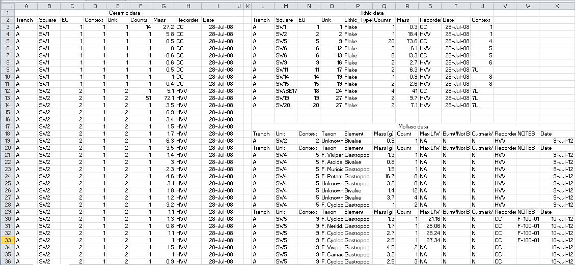
Figure 4.1: This screenshot shows archaeological data that is untidy for several reasons, including multiple tables on one sheet, multiple values in one column (e.g. SW1), and multiple header rows in a table
4.4 Cell organisation
At the most granular level of data collection is the individual spreadsheet cell or data entry field. Bad habits in data entry can require substantial time to fix before those data are suitable for analysis, and lead to errors in the results, regardless of what software yo use. Here I briefly review some of the common errors of cell organiation in the hope that if you are aware of them you might be motivated to avoid them in your data collection.
Choosing a good null value requires careful thought. Where you know that the value is zero, of course you should enter zero. But where the value was not measured, or could not be measured, you don’t want to enter zero because that implies that you know something about the value. You also don’t want to leave that field blank, because that could be interpreted as having missed to record that data. Blank cells are ambiguous - did the data collector skip that field by accident, or is were they not able to record a value for that field, or was the value zero? The best choice for the value we need in this situation is NA or NULL (White et al. 2013). NA is a good choice because it is a special (or reserved) word in the R language, so R can handle NAs easily. NULL might be better if your data uses NA as an abbreviation, such as “North America” (NULL is also a special word in R)
Another common pain point when moving from data collection to data analysis is where spreadsheets using formatting to convey information. For example, when a cell has coloured text or highlighting to indicate some extra information about that specimen or record. Related problems occur when bold or italic text is used to signal some important quality about the data. These types of are well-established in tables in publication, for example using bold to indicate values that are statistically significant. But at the point of data collection that use of cell and text decoration to convey information makes it very difficult to calculate on those values. It is always better to have another column to capture that information, rather than highlighting the cell or formatting the text.
knitr::include_graphics("images/messy_ktc_data_cell_decoration.png")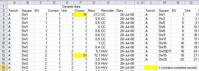
Figure 4.2: This screenshot shows spreadsheet formatting that is usesd to convey information. In this case, this yellow highlighing indicates that complete ceramic vessels were found in that level. A better approach would be to have a column called ‘complete_pots’, with values indicating the number of complete vessels in each unit
Related contaminants of spreadshet data include merged cells, cell comments and the inclusion of measurement units in a cell, such as the percent symbol. Merged cells can make it difficult to sort and filter data, and difficult move your into other programs for analysis. The proper place for comments is a ‘comments’ column, and units should be expressed in the column header, with only the same measurement unit used for every row in a column. When adding headers to your columns, take care not to include spaces, numbers, or special characters. A good alternative to spaces in column headings are underscore ("_“), for example,”Max_len_mm" or “MaxLenMM” is better than “Max len”, for a column of maximum length values in milimeters. Short or abbreviated field names (i.e. column headers) are often desirable during data collection to save screen space, but they may become confusing later when you revisit the data for analysis. So take care when devising column headers so they are not too ambiguous, and consider keeping a code book or data dictionary that pairs each column header with your description of the variable and how it was measured.
4.5 Summary
In this chapter we have reviewed principles, guidelines and rules for collecting data to maximise the ease of analysing that data in R. We considered some general principles of file organisation and file naming to keep your projects orderly and easy for you to keep track of your work over the duration of your project, as well as for others to inspect and resuse your work in the future. We explored methods to enhance the machine- and human-readability of your files. We introcuded the concept of ‘tidy data’ and some practical applications of this approach to spreadsheets. We noted were data are often untidy because of how they are collected, but proposed some rules to ensure data are as tidy as possible at the moment of collection. Finally we looked at the individual cell or field to identify some bad habits that are often seen in other people’s data. We proposed some simple rules for data entry into spreadsheet cells (i.e. sensible null values, not using formatting as data, not merging cells, etc.). The overarching concept is to excersice restraint when working with spreadsheets, and resist the temptation to engage all of its features. Be mindful of the downstream use of your data, by you in R, and by others in other softare environments. We can’t optimise our data collection for every possible data anlaysis situation, but with a few rules we can improve the organisation of our data to make it a lot easier to analyse it with other toolds.
References
Borer, Elizabeth T., Eric W. Seabloom, Matthew B. Jones, and Mark Schildhauer. 2009. “Some Simple Guidelines for Effective Data Management.” The Bulletin of the Ecological Society of America 90 (2). The Ecological Society of America: 205–14. https://doi.org/10.1890/0012-9623-90.2.205.
Ferris, Neal. 1999. “What’s in a Name? The Implications of Archaeological Terminology Used in Nonarchaeological Contexts.” Taming the Taxonomy: Toward a New Understanding of Great Lakes Archaeology, Edited by Ronald Williamson and Christopher Watts, 111–21.
Hampton, Stephanie E, Carly A Strasser, Joshua J Tewksbury, Wendy K Gram, Amber E Budden, Archer L Batcheller, Clifford S Duke, and John H Porter. 2013. “Big Data and the Future of Ecology.” Frontiers in Ecology and the Environment 11 (3). Ecological Society of America: 156–62. https://doi.org/10.1890/120103.
Kleindienst, MR. 2006. “On Naming Things.” Transitions Before the Transition. Springer, 13–28.
Noble, William Stafford. 2009. “A Quick Guide to Organizing Computational Biology Projects.” PLOS Computational Biology 5 (7). Public Library of Science: 1–5. https://doi.org/10.1371/journal.pcbi.1000424.
Strasser, C. A., and S. E. Hampton. 2012. “The Fractured Lab Notebook: Undergraduates and Ecological Data Management Training in the United States.” Ecosphere 3 (12). Ecological Society of America: 1–18. https://doi.org/10.1890/ES12-00139.1.
Sutter, Robert D., Susan B. Wainscott, John R. Boetsch, Craig J. Palmer, and David J. Rugg. 2015. “Practical Guidance for Integrating Data Management into Long-Term Ecological Monitoring Projects.” Wildlife Society Bulletin 39 (3): 451–63. https://doi.org/10.1002/wsb.548.
Volk, Carol J., Yasmin Lucero, and Katie Barnas. 2014. “Why Is Data Sharing in Collaborative Natural Resource Efforts so Hard and What Can We Do to Improve It?” Environmental Management 53 (5): 883–93. https://doi.org/10.1007/s00267-014-0258-2.
White, Ethan, Elita Baldridge, Zachary Brym, Kenneth Locey, Daniel McGlinn, and Sarah Supp. 2013. “Nine Simple Ways to Make It Easier to (Re)use Your Data.” Ideas in Ecology and Evolution 6 (2). https://doi.org/10.4033/iee.v6i2.4608.
Wickham, Hadley, and others. 2014. “Tidy Data.” Journal of Statistical Software 59 (10). Foundation for Open Access Statistics: 1–23.